


Comparison using the RSTMAC command
In a typical design procedure, you may want to make small changes to your model and compare the solutions you obtain from the new model to solutions from the original model. The RSTMAC command performs MAC calculations to compare the base and duplicate nodal solutions from two results files (.RST or .RSTP).
For cyclic symmetry analysis, the following applies:
The database must be saved after the solution is finished.
The mapping and interpolation method (
TolerN= -1) must be used.If nodes and/or elements are selected (using the NSEL and/or ESEL commands), the results of the mapping and/or the interpolation will show differences. If you want to perform the MAC calculation on a part of the model, you can use the ESEL command, but ensure you select the elements of the base sector as well as those of the duplicate sector. All the selected element nodes must also be selected (NSLE).
The modes obtained after a modal analysis for a cyclic symmetric structure are repeated when the harmonic index is greater than zero. In this case, the MAC values table is merged to allow solutions matching. This merging consists of summing and averaging the MAC values of the repeated frequencies.
This procedure is described fully in Comparing Nodal Solutions From Two Models or From One Model and Experimental Data (RSTMAC) in the Basic Analysis Guide.
Comparison using the MAXCYCMODE command
Due to the cyclically symmetric geometry, cyclic modes may come in pairs having the same frequency. This leads to an inherent indeterminacy in the mode shape orientations (travelling wave mode). These modes may exhibit a different phase angle at each solve and may also be different compared to the equivalent 360° model. However, the combination of the two modes is unique and can be used to compare solutions. The MAXCYCMODE command is a postprocessing tool that combines both modes of the pair and finds the maximum value of displacement or stress over the nodes of the travelling wave mode. This value can then be compared to the maximum of another set of mode pairs at the same frequency that is calculated in a separate solution from either:
A different model, for example comparing a cyclic symmetry analysis with a full 360° model.
The same model solved under different conditions, for example with a different frequency range or run on a different machine.
If the maximum values calculated using MAXCYCMODE for the two solutions are equal, you have mathematical evidence that the mode pair combinations and their respective models (or solutions) are equivalent.
The MAXCYCMODE command can be used on any mass normalized mode pairs at the same frequency that are computed in a modal analysis (ANTYPE,MODAL) of a cyclically symmetric system modeled in any of the following ways:
A cyclic symmetry model generated from the CYCLIC command as described in this guide.
A cyclic symmetry model generated under the multistage approach using the MSOPT and CECYCMS commands (See Multistage Cyclic Symmetry Analysis Guide).
A cyclically symmetric model generated without imposing symmetry boundary conditions (full 360° model).
If the model generated using the CYCLIC command has been cyclically expanded (/CYCEXPAND,,ON), issuing MAXCYCMODE will turn off the expansion (/CYCEXPAND,,OFF). Therefore, you must reissue /CYCEXPAND,,ON if cyclic expansion is required after issuing MAXCYCMODE.
The following example shows how to use MAXCYCMODE to compare a cyclic symmetry model generated from the CYCLIC command with a cyclic symmetry model generated under the multistage approach with a single stage using the MSOPT and CECYCMS commands.
Example 3.4: MAXCYCMODE to Compute the Maximum Results Value of Cyclic Mode Pairs
The following solution snippets demonstrate one possible use of the MAXCYCMODE command. Two inputs are run on the same geometric sector. The first solution uses the CYCLIC command to perform a cyclic symmetry analysis. The second solution uses the combination of MSOPT and CECYCMS to perform a multistage cyclic symmetry analysis on a single stage. Both solutions have mode pairs at the same modal frequency. The MAXCYCMODE command is used to determine if the mode pairs in the first solution are equivalent to the mode pairs in the second solution. Note that the MAXCYCMODE command uses:
Solution 1 snippets (CYCLIC):
/PREP7
…
CYCLIC
…
FINI
/SOLU
…
modopt,lanb,12
cycopt,hindex,HInd
…
solve
FINISH
/ POST1
MAXCYCMODE,1,1,'REAL',1,2,'REAL','USUM',6        !* Compute the max of the mode pair; last value is required when used with CYCLIC command
SET,1,1
PLNSOL,U,SUM     !* Visualize mode 1
SET,1,2
PLNSOL,U,SUM     !* Visualize mode 2

Solution 2 snippets (MSOPT/CECYCMS):
/PREP7
…
MSOPT,new,stag1,HInd
CECYCMS
…
FINI
/SOLU
…
modopt,lanb,12
…
solve
FINISH
/ POST1
MSOPT,EXPA,ALL,ALL                          !* Expansion needed before the macro for a multistage model
MAXCYCMODE,1,1,'REAL',1,2,'REAL','USUM'     !* Compute the max of the mode pair
SET,1,1
PLNSOL,U,SUM     !* Visualize mode 1
SET,1,2
PLNSOL,U,SUM     !* Visualize mode 2
Figure 3.4: Displacement vector sum results from MSOPT/CECYCMS solution at modal frequency = 278.385 Hz.
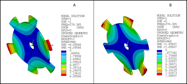
In this example, the four modes are similar, but their clocking angles are different. The maximum from MAXCYCMODE is exactly equal to 8.09980779 for both cases, which proves that the different modeling approaches are equivalent.