7.3. Example Submodeling Analysis Input

The following example submodeling analysis input listings are available:

7.3.1. Submodeling Analysis Input: No Load-History Dependency

The following example submodeling input does not include load-history dependency:

!  Start with coarse model analysis:
/FILNAME,coarse       ! Jobname = coarse
/PREP7                ! Enter PREP7
...
...                   ! Generate coarse model
...
FINISH

/SOLU                 ! Enter SOLUTION
ANTYPE,...            ! Analysis type and analysis options
...
D,...                 ! Loads and load step options
DSYMM,...
ACEL,...
...
SOLVE                 ! Coarse model solution
                      ! Results are on coarse.rst (or rmg, etc.)
SAVE                  ! Coarse model database file coarse.db
FINISH

!  Create submodel:
/CLEAR                ! Clear the database (or exit program and re-enter)
/FILNAME,submod       ! New jobname = submod
/PREP7                ! Re-enter PREP7
...
...                   ! Generate submodel
...

!  Perform cut-boundary interpolation:
NSEL,...              ! Select nodes on cut boundaries
NWRITE                ! Write those nodes to submod.node
ALLSEL                ! Restore full sets of all entities
NWRITE,temps,node     ! Write all nodes to temps.node (for
                      !   temperature interpolation)
SAVE                  ! Submodel database file submod.db
FINISH

RESUME,coarse,db      ! Resume coarse model database (coarse.db)
/POST1                ! Enter POST1
FILE,coarse,rst       ! Use coarse model results file
SET,...               ! Read in desired results data
CBDOF                 ! Reads cut-boundary nodes from submod.node and
                      !   writes D commands to submod.cbdo
BFINT,temps,node      ! Reads all submodel nodes from temps.node and
                      !   writes BF commands to submod.bfin (for
                      !   temperature interpolation)
FINISH                ! End of interpolation

RESUME                ! Resume submodel database (submod.db)
/SOLU                 ! Enter SOLUTION
ANTYPE,...            ! Analysis type and options
...
/INPUT,submod,cbdo    ! Cut-boundary degree-of-freedom specifications
/INPUT,submod,bfin    ! Interpolated temperature specifications
DSYMM,...             ! Other loads and load step options
ACEL,...
...
SOLVE                 ! Submodel solution
FINISH

/POST1                ! Enter POST1
...
...                   ! Verify submodel results
...
FINISH

7.3.2. Submodeling Analysis Input: Load-History Dependency

The following example submodeling input includes load-history dependency:

!  Start with coarse model analysis:
/FILNAME,coarse       ! Jobname = coarse
/PREP7                ! Enter PREP7
...
...                   ! Generate coarse model
...
FINISH
/SOLU                 ! Enter SOLUTION
ANTYPE,...            ! Analysis type and analysis options
...
D,...                 ! Loads and load step options
DSYMM,...
ACEL,...
...
SOLVE                 ! Coarse model solution
                      ! Results are on coarse.rst (or rmg, etc.)
SAVE                  ! Coarse model database file coarse.db
FINISH
!  Create submodel:
/CLEAR                ! Clear the database (or exit program and re-enter)
/FILNAME,submod       ! New jobname = submod
/PREP7                ! Re-enter PREP7
...
...                   ! Generate submodel
...
!  Perform cut-boundary interpolation:
NSEL,...              ! Select nodes on cut boundaries
NWRITE                ! Write those nodes to submod.node
ALLSEL                ! Restore full sets of all entities
NWRITE,temps,node     ! Write all nodes to temps.node (for
                      !   temperature interpolation)
SAVE                  ! Submodel database file submod.db
FINISH
RESUME,coarse,db      ! Resume coarse model database (coarse.db)
/POST1                ! Enter POST1
FILE,coarse,rst       ! Use coarse model results file
SET,...               ! Read in desired results data
CBDOF                 ! Reads cut-boundary nodes from submod.node and
                      !   writes D commands to submod.cbdo
BFINT,temps,node      ! Reads all submodel nodes from temps.node and
                      !   writes BF commands to submod.bfin (for
                      !   temperature interpolation)
SET,...               ! Read in another desired results data
CBDOF                 ! Reads cut-boundary nodes from submod.node and
                      !   writes D commands to submod.cbdo
BFINT,temps,node      ! Reads all submodel nodes from temps.node and
                      !   writes BF commands to submod.bfin (for
                      !   temperature interpolation)
...                     This(SET,CBDOF,BFINT)can be repeated many time 
FINISH                ! End of interpolation
RESUME                ! Resume submodel database (submod.db)
/SOLU                 ! Enter SOLUTION
ANTYPE,...            ! Analysis type and options
...
/INPUT,submod,cbdo    ! Cut-boundary degree-of-freedom specifications
/INPUT,submod,bfin    ! Interpolated temperature specifications
DSYMM,...             ! Other loads and load step options
ACEL,...
...
TIME
SOLVE                 ! Submodel solution of first steps
/INPUT,submod,cbdo    ! Cut-boundary degree of freedom from another set
/INPUT,submod,bfin    ! Interpolated temperature from another set
TIME
SOLVE                   SOLVE as another load step
…..                     This (/INPUT..SOLVE) can be repeated many time
FINISH
/POST1                ! Enter POST1
...
...                   ! Verify submodel results
...
FINISH

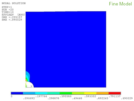
Following is a simple model of a plate with a hole in its middle, with applied displacements in the x direction. To simulate load-history dependency, cut boundary conditions are done at different substeps of the coarse-mesh analysis, then applied as different load steps in the submodeling analysis. The material is assumed to be rate-dependent anisotropic plastic with isotropic hardening.

The problem is solved via the coarse-mesh model, the submodel, and the fine-mesh model, as shown in this figure:

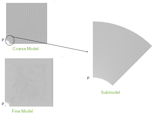
Figure 7.9: Coarse-Mesh Model, Submodel, and Fine-Mesh Model

Both the coarse-mesh model and the fine-mesh model are solved in 20 substeps. The fine-mesh model yields a benchmark solution for comparison purposes.

The submodel analysis is performed in four solutions, as follows:

With cut-boundary conditions at only the last substep of the coarse-mesh analysis, solved in one load step with 20 substeps.
With cut-boundary conditions at five substeps (that is, at every four substeps) of the coarse-mesh analysis, solved in five load steps each with about four substeps.
With cut-boundary conditions at 10 substeps (that is, at every two substeps) of the coarse-mesh analysis, solved in 10 load steps, each with about two substeps.
With cut-boundary conditions at all 20 substeps of the coarse-mesh analysis, solved in 20 load steps, each with about two substeps.

The specified load steps and substeps make the size of the substep in submodel solutions close to those in whole-model solutions.

The following figure shows the equivalent plastic strains at point P in each solution:

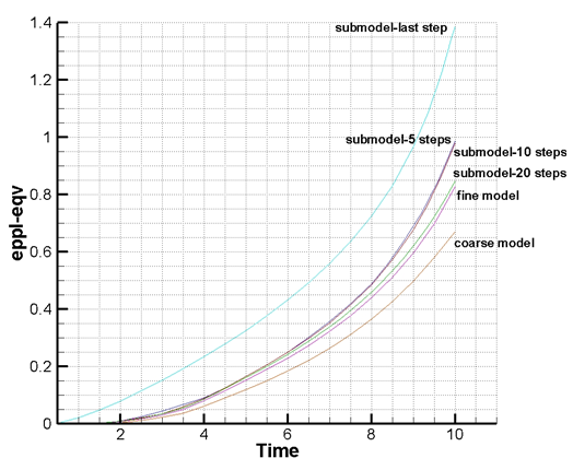
Figure 7.10: Equivalent Plastic Strain Through Various Cut-Boundary Conditions and Load Steps

When boundary conditions are cut at more substeps, the results are closer to the fine mesh (the correct solution).

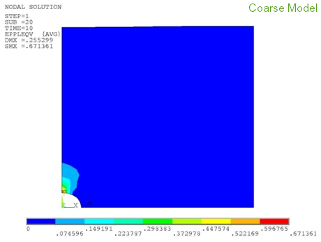
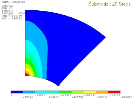
The following figure shows the contour plots of equivalent plastic strain at the end of loading for each of the four solutions:

Figure 7.11: Equivalent Plastic Strain Distributions in a Submodeling Analysis with Load-History Dependency

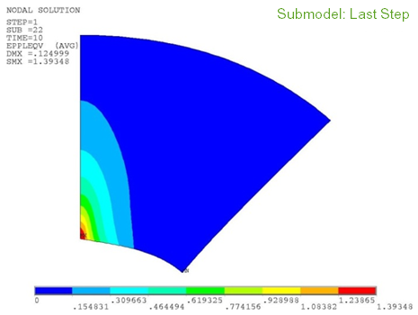The results with 20 boundary-condition cuttings most resemble the fine-mesh model.

As the example indicates, boundary conditions should be cut from more substeps of the coarse solution to reflect load-history dependency more accurately.