This example uses the axially-symmetric acoustic element, FLUID244, to represent acoustic radiation from a circular piston in a water medium.

The figure below shows the two-dimensional model, including a piston structure and the fluid domain enclosed by radiation elements, FLUID129.

Figure 13.15: 2D Model of Circular Piston in Water Medium

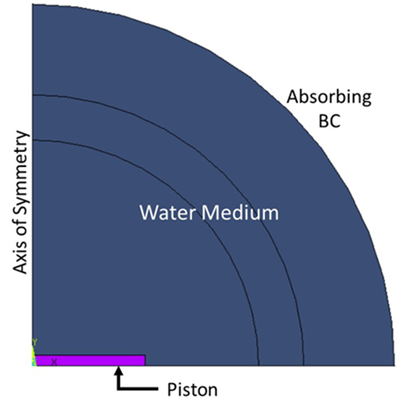
The Dirichlet boundary condition is applied to the piston surface for the displacement, and the equivalent source boundary condition (SF,,MXWF) is used for the radiation sources. The fluid-structure interface is applied on the surfaces between the structure and the fluid domain.

In reference [1], the theoretical acoustic pressure is given by:

where denotes the radius of the piston cylinder and is wavelength. represents the velocity of the piston.

The water mass density ()= 1000 kg/m³ and speed of sound (c)= 1500 m/s.

The coupled harmonic analysis solves the fluid domain. After the computation of far-field propagation, PRFAR and PLFAR commands generate acoustic pressure and sound pressure level (SPL) output for different observer points.

/batch
/prep7
KA=4
DIM_RAD   = 0.125
K0=KA/DIM_RAD
MAT_DENS  = 1000
MAT_SONC  = 1500
FREQUENCY = K0*MAT_SONC/(2*acos(-1))
WAVENUM   = 2*acos(-1)*FREQUENCY/MAT_SONC
WAVELENG  = MAT_SONC/FREQUENCY
DIM_BUFF  = 0.3
DIM_MEAS  = 0.4
un        = 0.001
DIM_ESIZE = WAVELENG/12
!
! Define Elements and Materials
et,1,244,,0,1                    ! 2nd-order Axisymmetric element
et,3,129,2,,1                    ! High order radiation element (Axisymmetric)
et,2,183,,,1
r,1,20e-6
r,2,DIM_MEAS
mp,dens,1,MAT_DENS
mp,sonc,1,MAT_SONC
mp,ex,2,1.44e11
mp,dens,2,7700
mp,nuxy,2,0.35
!
! Generate Areas
cyl4,0,0,0,0,DIM_RAD*2,90
rect,0,DIM_RAD,0,DIM_RAD/10
asba,1,2,,dele,keep
cyl4,0,0,DIM_RAD*2,0,DIM_BUFF,90
cyl4,0,0,DIM_BUFF,0,DIM_MEAS,90
alls
aglue,all
alls
!
! Generate Mesh
type,1
mat,1
!real,1
esize,DIM_ESIZE
asel,u,,,2
amesh,all
alls
type,2
mat,2
asel,s,,,2
amesh,all
alls
nummgr,all
alls
csys,2
nsel,s,loc,x,DIM_MEAS
type,3
mat,1
real,2
esize,DIM_ESIZE
esurf
alls
!
! Assign displacement
csys,0
nsel,s,loc,x,0,DIM_RAD
nsel,r,loc,y,0
d,all,uy,un
alls
!
! MXWF BCs
csys,2
nsel,s,loc,x,0,DIM_RAD*2
esln,s,1
nsel,s,loc,x,DIM_RAD*2
sf,all,mxwf
alls
csys,0
!
! Solution
/solu
antype,harmic
harfrq,1000,5000
nsub,4
kbc,1
solve
finish
!
/post1
csys,0
hfsym,0,,shb
hfang,,0,360,0,90
/output
set,1,1
prfar,pres,splc,0,90,9,90,90,1,20,,
set,1,2,
prfar,pres,splc,0,90,9,90,90,1,20,,
set,1,4
prfar,pres,splc,0,90,9,90,90,1,20,,
finish
!
! Postprocessing
/post1
hfsym,0,,shb
hfang,,0,360,0,90
plfar,pres,splc,0,90,9,90,90,1,20,2.e-5,,,,,all,2000,5000,
finish
!
! Update KA
KA=10
DIM_RAD   = 0.125
K0=KA/DIM_RAD
MAT_DENS  = 1000
MAT_SONC  = 1500
FREQUENCY = K0*MAT_SONC/(2*acos(-1))
!
! New solution
/solution
antype,harmic
harfrq,FREQUENCY
nsub,1
kbc,1
solve
finish
!
/post1
hfsym,0,,shb
hfang,,0,360,0,90
/output
set,1,1
/title,  SPL-Phi for KA=10
plfar,pres,splc,-5,5,100,0,10,100,0.0001,,,,,1,1,,,plxy
plfar,pres,splp,0,180,180,90,90,1,20,2.e-5,,,,,all,2000,20000,
finish

The sound pressure level at various angles is demonstrated in the figure below for 3 different frequencies (2000 Hz, 3000 Hz and 5000 Hz). The non-dimensional radial distance is 160.

Figure 13.16: Phi Angle vs. Sound Pressure Level Comparison of Theoretical and Mechanical APDL Results

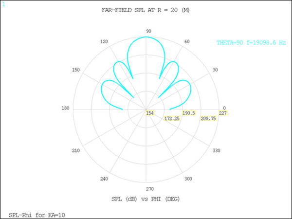
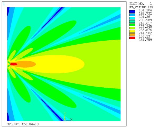
To represent a similar computation to reference [1], the value is set to 10. The driven far-field propagation outputs show good agreement with the beam pattern in the reference.

Figure 13.17: Sound Pressure Level in Polar Coordinates for ka=10

Figure 13.18: Sound Pressure Level Distribution on XY Plane