Theory of Order Analysis
The order analysis computed in Ansys Sound: Analysis and Specification is based on the Synchronous Order Analysis method.
Starting from the temporal waveform (the original signal as samples vs. time) and its associated synchronous RPM Profile, the signal is transformed to obtain a new version of its evolution as a function of an equally spaced vector of number of cycles. In other words, the signal is resampled at a tachometric constant step, meaning a constantly sampled number of revolutions vector.
In what follows, "one revolution" (as used in the term "revolutions per minute", or "rpm") is referred to as "a cycle".
- Consider a signal (named "S") as a function of time, that has a constant sampling frequency. This signal may be an acoustic sound, a vibration, etcetera. Also consider the signal's associated synchronous RPM profile (named "RPM").
- From the RPM, the starting times of each cycle are known. Build a vector (named "C") of the number of cycles, including regular subdivisions of the cycle. If "N" is the number of regular subdivisions of the cycle (the number of points per cycle), then the vector C will have N times per cycle. This means that every N points, a new cycle is starting. Thus, from vector C and the RPM, the times associated to C values are known.
- Knowing vector C and signal S, a synchronous resampling is performed. The signal S is resampled toward this vector of N number of points per cycle. An anti-aliasing filter is used during the process if needed. This new signal is named "RS", and it contains the amplitudes (from signal S) corresponding to the times associated to the cycle numbers (the vector C).
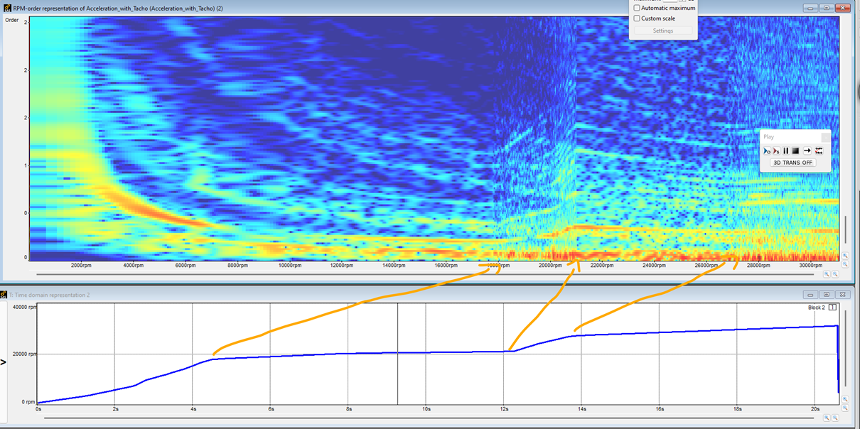
- The "order vs. time" representation is the colormap display of the level as a function of time and order number. See Changing the Representation Display (ansys.com) for more information.
- The "order vs. rpm" representation is the colormap display of the level as a function of rpm and order number. See Changing the Representation Display (ansys.com) for more information.
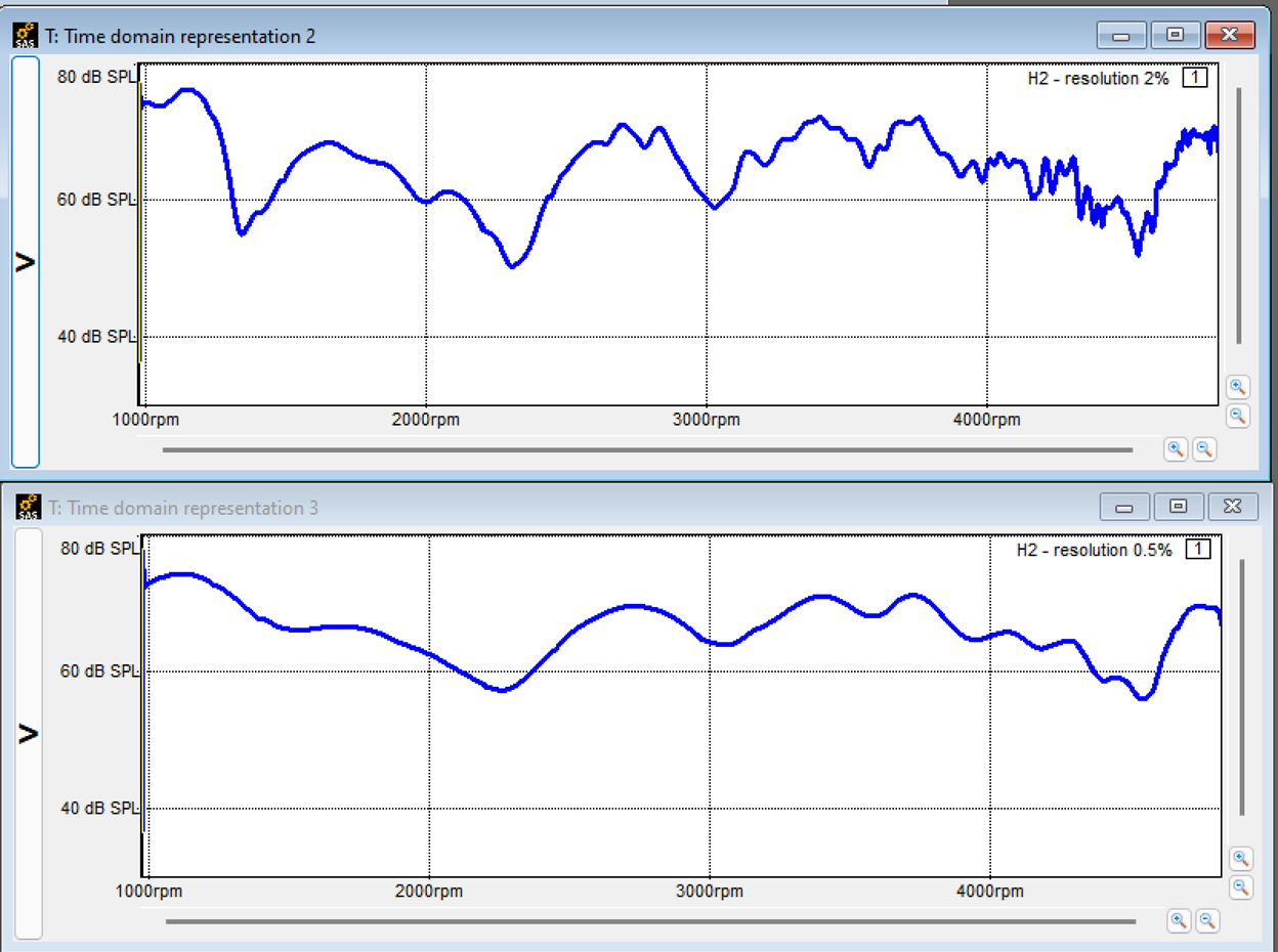
- The individual order level is the level of a specific order, and can be displayed as a function of time or rpm. See Displaying Order Levels in a Graph (ansys.com) for more information.
The "order vs. time" and "order vs. rpm" displays are colormap displays that are directly issued from the spectrogram of the synchronous sampling signal RS. The spectrogram of RS is calculated using a short-time Fourier transform (the same as the other spectrograms used in Ansys Sound: Analysis and Specification).
Highest order for order view: This parameter (named "Omax") is the maximum order rank that you intend to be able to analyze. It has an influence on the number of cycles N that will be used for the synchronous sampling. The software uses the value N = 2 x Omax + 1, so that the Nyquist theorem is fulfilled for analyzing order Omax.
Hence, if you are interested in analyzing the orders up to the 20th one, then 41 points per cycle will be used for the sampling.
Resolution for order display: This parameter is the resolution of the analysis on the orders axis, in percent of the order.
Due to the Heisenberg uncertainty principle, the finer the Order analysis resolution is, the coarser the resolution of the axis of cycles number is. Inversely, the coarser the resolution is on the order axis, the finer the resolution is on the cycles axis.
For example, the image on the left shows the "order vs. rpm" display with a resolution of 4% of order. The image on the right shows the "order vs. rpm" display with a resolution of 0.5% of order.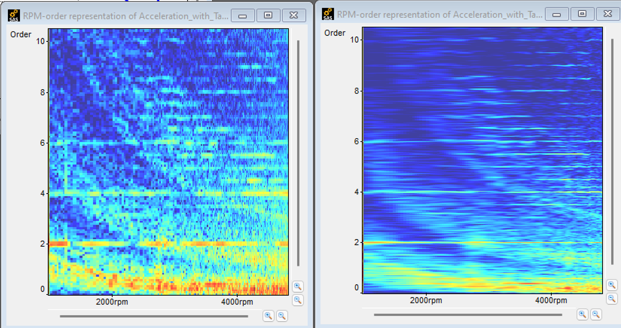
The Individual order level is calculated from this STFT. The above-mentioned parameters have an influence on the result of this calculation.
The Order analysis width also has influence. The order analysis width is a parameter used for the estimation of the "level vs. cycle" number of a specific order. For example, if you want to estimate the level of the order #2, using an order analysis width of 20% of order, the calculation of the level will be done from the STFT of RS, by integrating (that is, summing) all the level points contained in the order band that goes from 2-0.1 to 2+0.1 (that is, the band of orders around order 2: [1.9, 2.1]).
Obviously, the shape of the resulting curve depends on the parameter Order analysis resolution in percent of order (as stated before for the colormap). The finer this resolution is, the smoother the curve is (but the level is estimated using more cycles), and inversely the coarser the resolution is, the more erratic the shape of the curve is (but the level is estimated using fewer cycles). For more information, refer to Displaying Order Levels in a Graph (ansys.com).