Set up and Run an Array Simulation

There are some changes in the GUI for setting up the adaptive simulation for designs with a virtual array and if the design uses 3D components However, the solution quantities of the virtual cells will be available for convergence setup (In both adaptive and interpolating sweep). There are no changes in the way convergence information is presented on the Convergence tab of the Solution Display panel.

If your design contains a virtual array and/or 3D Components, the Solution setup can have some differences.

• If an array contains 3D Components, the Solution Setup Options tab contains a Skip 3D Component Array Solve During adaptive Passes option.
  
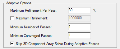
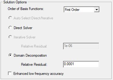
  This option is on by default. The mesh for each component is independently adapted, which significantly improves the performance compared to full array adapt with minimum lost of accuracy. Even it is a composite design, the solver still adapts each component as non-composite during component adapt. As a result, even though it's showing Max Delta Normalized Power due to UI constraints, the underlining calculations are all based on Max Mag Delta S from each component.
• The Solution Option for Domain Decomposition is automatically checked. You can choose Direct Solver. Iterative Solver options are disabled. The domains are UI defined through the array definition, not solver defined domains.
  
• Set up the distributed processor workgroup. Designs with arrays require HPC licenses.
• General Setup for Virtual Array Simulation for Matrix Convergence, if you choose Selected Entries.
• Interpolating Sweep Advanced Options for Array Simulation
• Fast sweep is not supported.
• You can also set up the expression cache at solve setup. The expression cache interface for accessing array elements is the same as those used in report setup.
• Use the Active Cells tab on the Regular Array dialog or 3D Component Array dialog to designate which cells are active or passive for a simulation. You can make All Active, All Passive or select which cells are active or passive. The more active cells there are for a simulation, the more processing is required. By default, clicking the corresponding array elements toggles the current selection, You can also choose the Mouse makes cell setting to click for Active or Passive, whichever is most convenient. Clicking on a row or column number applies the mouse click command to all cells in that row or column. Dragging the cursor over cells performs the current operation on them.

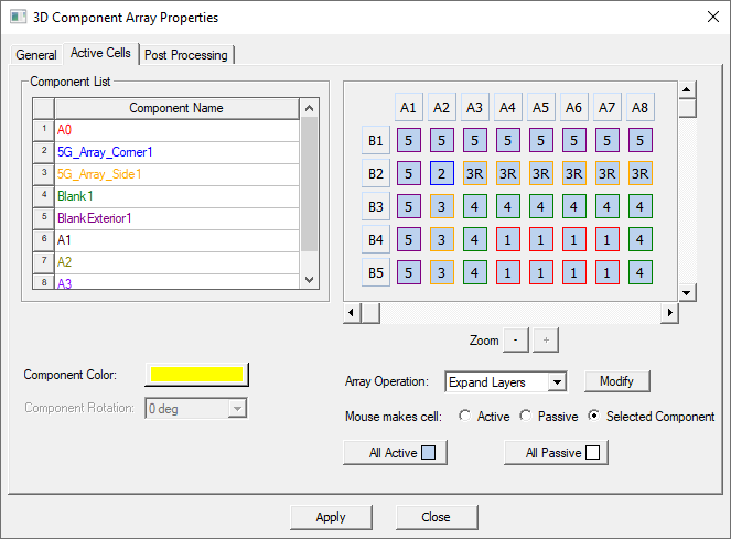
It is important to understand the impact of passive ports on antenna parameters. For accepted power calculations, passive ports are not included when computing the total power passing through the union of all port surfaces. This means that the passive ports can be viewed as a loss mechanism for the device and it is not equivalent to viewing the passive ports as active ports with zero excitations.

• Report setup for Arrays.

The solution/matrix quantities are grouped by category. The entries in each category are listed according to their [row, column] order in the corresponding matrix.

The entry in [row1, column1] will be listed first, followed by

[row1, column2], … [row1, columnN], [row2, column1], …

[row2, columnN], … [rowN, columnN]. Note that the [row, column] order of each entry in the matrix is controlled by the 'Matrix' order as specified by user.

The existing "Filter" capability can help locate the desired quantity from the potentially very long list.

Beta Feature: Parallel Component Mesh Adapt

If Skip 3D Component Array Solve During Adaptive Passes is selected and you enable the Beta feature Parallel Component Mesh Adapt, if a design contains multiple 3D Components in an array, and is run through HPC, the Solution Profile can show multiple hf3d solvers for frequency solves.

Beta Feature: Composite Subarray in HFSS Finite Array Design

A composite excitation is simply a specific superposition of defined sources. Using composite excitations can speed up analysis and reduce storage requirement for fields when there are many sources, and you are only interested in a few combinations of those sources (for example, for 5G antennae).

This feature resembles the composite solution type in which all source excitations are combined into a single source. Here, however, you can combine a subset of sources into a single source. This feature supports multiple, named, subsets of sources. When solved, each subset presents as a single source to the reporter. Each combined source (namely composite group) is accessible from Edit Sources to control its magnitude and impedance.

For an HFSS design with a finite array, and the Beta Feature Composite Subarray in Network Analysis enabled you can access the composite subarray functionality by right-clicking on the Array Item in the Project tree and selecting Composite Subarray in the menu.

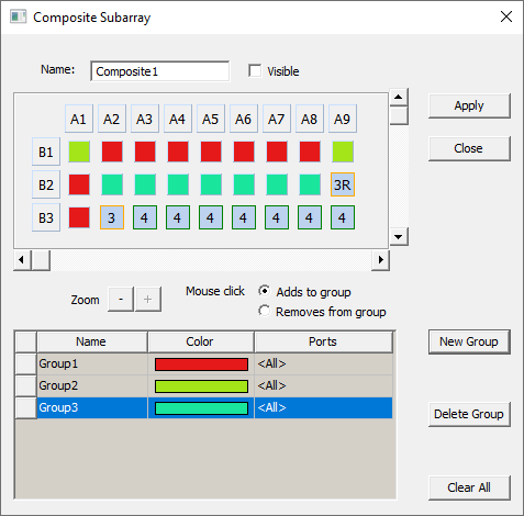
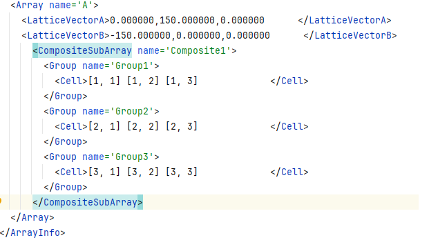
In the Composite SubarrayArray dialog, you can create/edit/delete composite groups and assign array cells to composite groups in a similar way that you defined the array itself. If the design includes an existing subarray, it is depicted in the dialog. Notice that the boundary colors for the defined cell are independent of those applied to define each new group. You can click on individual cells to assign them to the currently active group.

You can click on individual cells to assign them to the currently active group, or click on the Row or Column number to assign that row or column. You can resize the dialog and use the vertical and horizontal scroll bars to view array cells for selection. Click the New Group for a new one which will be given new colors, and by default, an incremented name.

Click Apply to activate the Group Assignment in the Modeler window display. Once you have defined a subarray, it appears in the Project tree.

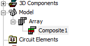
You can right-click on the Composite subarray to view the Properties window, and to Visualize Current Subarray assignments in the Modeler window. Once the composite array is defined and is set to visible, each composite group would be visualized using a unique color overlay in the modeler.

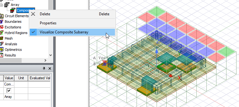
Note that in the example figure, the blue color for the cells in Row three in the dialog has been applied to the cells in the Row 3 modeler window.

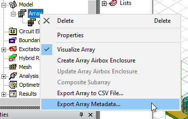
After a composite subarray design is solved, you can export array metadata by right clicking the array item in project tree:, you can right-click on Array to Export Array Metadata.

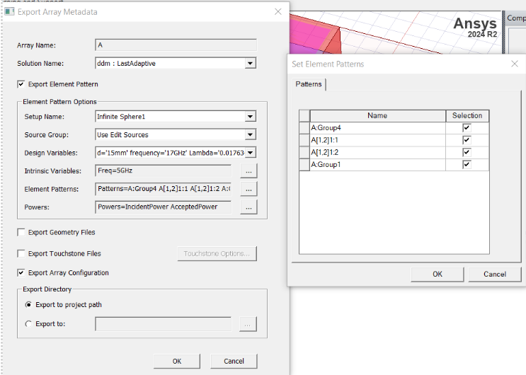
In the Export Array Metadatadialog the element pattern selection shows composite groups instead of individual ports.

For designs that Link from Driven Modal Design to SBR+, the Phase Reference Setting dialog also offers choices for composite groups if you want to specify unique phase reference for each group.

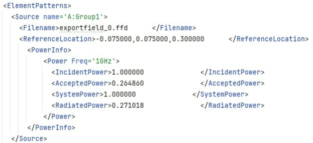
Similarly, the powers in the export metadata header file would clearly show the group names and group element patterns (i.e., only this composite group is excited). For example:

Composite Array Post-Processing

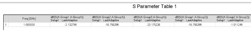
Once a finite array design with composite array is solved, post-processing treats each composite group as if it is a single excitation. For example, in an S-parameter table, you can examine the S parameter between each group in modal solution reporter and matrix display, where the composite group name is shown instead of an individual port.

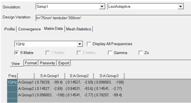
The Matrix Data tab of the Solution Data does the same thing, showing composite group names, rather than port names.

For field post-processing, the Edit Source dialog includes the settings of each port, and each group has its own scaling factor, which can be defined in the Composite Excitation tab.

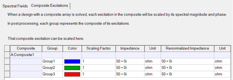
As with an individual port, you can also define impedance and renormalized impedance for composite groups, but the underlying logic is slightly different.

Due to limitations you must explicitly define the Z₀ of composite group, and the renormalized impedance will be used as Z₀ (i.e., composite group always applies post-processing effects). On the other hand, the concept of "Impedance" is introduced solely to account for the matrix renormalization effect (e.g. for S matrix normalization) which is based on the ratio of impedance and renormalized impedance.

For example, a composite group with A impedance and B renormalized impedance can be seen as an individual port with A impedance and B renormalized impedance, with renormalization effect turned on. Therefore, if you do not want any renormalization for composite group, you must simply ensure that A and B are the same and match the expected impedance value.

The impedance and renormalized impedance is only used for matrix quantity (e.g., S parameter, Z₀) but not for fields results. The "Include Post Processing Effects" option is disabled to reflect this concept.

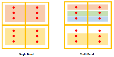
Multi-band Composite Subarray

HFSS support multiple composite excitations within a given design, along with S-parameters between these excitations. A composite excitation is a specific superposition of defined sources. Leveraging composite excitations can significantly enhance analysis efficiency and reduce storage requirements for field data. A Beta feature allows multi-band composite subarrays, addressing realistic and complex scenario requirements. If array cells have multiple ports, you can further subdivide existing composite groups to include specific ports, as shown in the figure below.

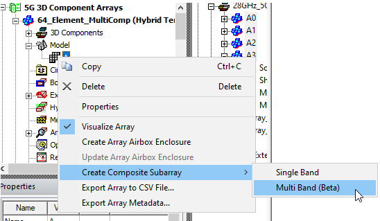
When feature is enabled, and the design has an array and multiple ports defined click the array right-click menu to select Create Composite Subarray>Multi Band (Beta):

This opens the Composite Subarray dialog, with Rows and Columns appropriate to the design to select which port(s) to be included in a composite group. The interface differs from the Single Band version in that it contains a Ports column with a field that allows you to select single or multiple ports to define additional bands.

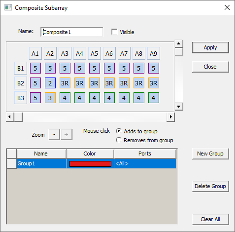
Right-click on the Ports for the group to see a drop down with the available ports listed.

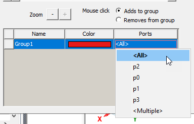
You can select either all ports (making a single-band composite subarray), one port or <Multiple> for a subset of ports.

You can define additional groups and edit the contents of groups.