Defining Nonlinear Material Properties

When adding a new material or editing an existing material, the material properties list contains several editable fields.

To define nonlinear material properties:

1. From the View/Edit Material window, click a property's Type field and select Nonlinear.

   From the Value field, one of the following buttons appears, depending on the property:

   • B-H Curve – for nonlinear relative permeability. See: B-H Curves below.
   • D-E Curve – for nonlinear relative permittivity. See: D-E Curves below.
   • J-E Curve – for nonlinear bulk conductivity. See: J-E Curves below.

   

2. Click an appropriate button.

   The [BH / DE / JE] Curve window appears.

   Each of these windows contains a Coordinates table where you can define curve values, as well as buttons for importing and exporting datasets. If imported data are swapped in the Coordinates table, use the Swap X-Y Data button to correct this.

3. Define the coordinates using either the Coordinates table or Import Dataset. The curve previews in the graph to the right.
4. When you are finished, click OK.
5. Click OK again to close the View/Edit Material window.

B-H Curves

For nonlinear relative permeability, you must specify magnetization characteristics using BH curves, where B is total magnetic flux density and H is the magnetic field. SIwave can also model temperature dependencies of the nonlinear material property when you provide two or more temperature-dependent BH curves.

To define a single B-H curve:

1. Select whether B values are Normal or Intrinsic.

   Important:

   • For a Normal curve, the slope of the curve can not be less than that of free space anywhere along the curve.
   • For an Intrinsic curve, the slope of the curve can not be less than 0.
   • Normal curves are extrapolated; Intrinsic curves are not.
2. Use the Units drop-down menus to define units for B and H.
3. Enter B and H values in the Coordinates table or Import Dataset.

   Note:

   • The initial value of B must be 0.
   • The value of B must increase along the curve.
   • The slope of the last two user-defined data points is used to extrapolate the BH curve. Therefore, you must enter enough points for accurate representation.
4. Preview the graph to ensure it looks correct.
5. Click OK.

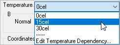
To define temperature-dependent BH curves:

1. Use the Temperature drop-down menu to select Edit Temperature Dependency.

   The Edit Temperature Dependency window appears.

   

2. Select the Temperature Dependent check box and add rows for the temperatures at which you wish to define BH values.
3. Click OK.
4. Back in the BH Curve window, use the Temperature drop-down box to select each temperature.

   

5. Define each temperature's BH values using the Coordinates field.
6. Click OK.

D-E Curves

For nonlinear relative permittivity, you must specify magnetization characteristics using DE curves, where D is the electric flux density and E is electric field strength.

To define a D-E curve:

1. Use the Units drop-down menus to select units for D and E.
2. Enter values using the Coordinates table or Import Dataset.

   Note:

   • The initial value of D and E must be 0.
   • The slope of the curve cannot be less than 0.
   • The slope of the last two user-defined data points is used to extrapolate the DE curve. Therefore, you must enter enough points for accurate representation.
3. Click OK.

J-E Curves

For nonlinear bulk conductivity, you must specify the J-E Curve, where J is the current density and E is the electric field.

To define a J-E curve:

1. Use the Units drop-down menus to select units for J and E.
2. Enter values using the Coordinates table or Import Dataset.

   Note:

   • The initial value of J and E must be 0.
   • The slope of the curve cannot be less than 0.
   • The slope of the last two user-defined data points is used to extrapolate the JE curve. Therefore, you must enter enough points for accurate representation.
3. Click OK.