
Creating a New Report
Following is the general procedure for creating a new report:
- From the Maxwell 2D or Maxwell 3D menu or from the Project Manager tree, point to Results, and then select Create <type> Report and select Display Type for that template. The available Report Types depend on the simulation setup.
- In the Context section make selections from the following field or fields, depending on the design and solution type.
- Solution field with a drop down selection
list. This lists the available setups and sweeps. As a minimum, the LastAdaptive
solution and AdaptivePass solution is available to choose.
The AdaptivePass solution context can be selected to allow any value or parameter to be plotted versus the adaptive pass. This function is usually used to evaluate the convergence of the solution.
- For Transient projects only: Domain field with a drop-down selection list containing options for plotting vs time (Sweep Domain) or plotting vs frequency (Spectral Domain).
- For Transient projects only: Domain field with a drop-down selection list containing options for Average and RMS and Transient D-Q for electric machines. Click Machine Options to setup the machine specific parameters.
-
For Eddy Current projects only: Domain field with a drop-down selection list containing options for plotting vs frequency (Sweep Domain) or plotting vs time (Time Domain).
Matrix field with a drop-down selection list containing options for plotting matrix and reduce matrix parameters.
Note: In Maxwell Eddy Current designs, the user can create matrix parameters, which will cause the solver to produce an impedance matrix for the selected excitations. In addition, for the Eddy Current T-W solver, the user can group (wire) two or more excitations to one excitation in either a series or parallel connection referred to as a reduce matrix. The Matrix field appears only if a matrix entry is selected in the Parameter field. (Refer to Assigning a Matrix for information on creating a matrix and Assigning a Reduce Matrix for information on creating reduced matrix parameters for Eddy Current designs.)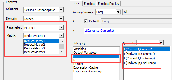
- Parameter field with a drop down selection list. Whether this field appears, and the parameters listed depend on the Solution type and the <type> selected.
- For Fields and Noise Vibration reports: Geometry field with a drop down selection list. This applies the quantity to a specific geometry.
- In the Y Component section, make selections for the following:
- Categories - depend on the Solution type and the design. For example, Magnetostatic categories include: Torque, Output Variables, Inductance, and other user-selectable solution parameters. Transient categories include: Loss, Output Variables, Variables, and others. Eddy current categories include Loss, Winding, End Connection, L (inductance), R (resistance) Z (impedance), and others.
- Quantities for Y are relative to the
selected category. For example, Loss quantities include CoreLoss, EddyCurrentLoss,
HysteresisLoss, and others.
Winding quantities include Flux Linkage, Induced Voltage, and others - depending on the winding type.
Note: The Quantity text field can be used to filter the Quantity list by typing in text, or by using the four predefined selections. This is useful if the Category selected produces a lengthy Quantities list. See Filtering Quantity Selections for the Reporter.
When the matrix is very large, the number of quantities can be correspondingly huge. Therefore, the Quantities field can optionally use a tree structure to divide matrix quantities into groups by their first element name. The initial display shows groups, without initially listing group members.
- Function list to apply to the Y quantities.
- The Y value field displays the currently
specified Quantity and Function. You can edit this field directly.
Note: Color indicates if an expression is valid.
- The Range Function button opens the Set Range Function dialog box, which applies currently specified Quantity and Function.
- In the X (Primary Sweep) section, make selections for the following:
- Select the Primary sweep from the drop down menu. By default All of the chosen sweep’s values are used. You can also select the browse [...] button to display a dialog box that lets you select particular sweep values, specify a range of sweep values (for Time sweeps), or Use all values (the default setting).
- The Families tab provides a way to select from valid solutions for sweeps where a simulation has multiple variables defined (for example, for a parametric sweep). If so, the variables other than the one chosen as the X (Primary sweep), are listed under the Families tab with columns for the variable, the value, and an Edit column with an ellipsis [...] button. See Using Families tab for Reports.
- Update Report settings:
- Real Time checked: enables real-time updates for all reports while the reports are being edited.
- Real Time unchecked: enables drop-down menu to Update All Reports or Update Report. Reports will only be updated with one of these user selectable update options or upon exiting the report dialog box. This can be useful if you expect a trace to take time to display. You can then add additional traces without having to wait.
- The Report dialog command buttons permit you create a new report with the settings you provide, or to modify an existing report.
- Output Variables – opens the Output Variables dialog box.
- Add Trace – this is enabled when you have created or selected a report. Add one or more traces to include in the report.
- Update Trace – updates the selected traces in a report based on further processing or changes.
- New Report – Adds a report to the Project Manager tree under the Results icon. The new Report is displayed in the Project Manager window.
- Options – opens the Report Setup Options dialog box. This contains a check box for using the advanced mode for editing and viewing trace components. This mode is automatic if the trace requires it. It also contains a field for setting the maximum number of significant digits to display for numerical quantities.
- Close – closes the Report dialog box.
- Click New Report to create a new report in the Project Manager tree.
- To speed redraw times for changed plots, perform a Save. This saves the data that comprises expressions. If you do not do a save of a changed plot, the changed version is not stored.
If you have created custom report templates (for example, including your company name or other format changes), you can also create a report based on that template by selecting Maxwell 2D, Maxwell 3D, or RMxprt > Results > Report Templates > PersonalLib > <templateName>. You can also make such changes the default for new reports by right-clicking a modified report and selecting Report Templates > Save Settings as default.
When you have selected the <type> and display type from the Results menu, the Report dialog box appears, with the Trace tab selected by default.
To select an X component that is different from the Primary Sweep, uncheck the Default field to enable the X field and browse [...] button. Click the browse [...] button to display the Select X Component dialog box. This lets you specify the X component as you do the Y; that is, in terms of Categories which define the selectable Quantities, and Functions to apply. After making selections, OK the dialog to assign the X component.
The report appears in the view window. It will be listed in the Project Manager tree under Results, with the default name based on the Report Category you selected, for example, Force Plot n or Output Variables Plot n. You can edit the plot names in the project tree and the plot header text in the report synchronizes. Traces within the report also appear in the Project Manager tree. Some plots may take time to complete. Performing a File > Save in such cases after the plot has been created will permit you to review the plot later without having to repeat the calculation time when you reopen the project later.