
Maxwell 3D Transient Solution Based on A-Phi Formulation
By default, the Maxwell 3D transient solver is based on T-W formulation, which is a powerful method for solving a wide range of low-frequency EM problems. However, there are some areas where the applicability of the method is limited – such as multiple (mixed) source excitations on a single conduction path and capacitive effect (displacement current). For simulation of such problems, the Maxwell 3D Transient A-F formulation (A-Phi in the Solution Type window) is a more suitable solution type.
Comparison of T-W and A-F Solvers
| T-W | A-F |
|---|---|
|
Solves second-order elements for magnetic B field |
Solves second-order F for electrical E field, and solves first-order A for magnetic B field. (In order to account the difference in the order of elements solved, increasing the mesh density in A- F should help achieve the same B field results as T- Ω.) |
|
Computational efficient for electric machines applications |
Computational efficient and flexible for ECAD PCB and electronics applications |
|
Does not support multi-terminals with mixed excitation types on the same conduction path |
Supports multi-terminals with mixed excitation types on the same conduction path |
|
Ignores displacement current |
Can consider capacitive effects (displacement current) |
|
Supports all advanced material modeling |
Limited advanced material modeling capabilities |
|
Easy handling of motion due to only scalar potential for the motion coupling |
Does not support motion |
For more information on the Transient A-F formulation, refer to the following sections:
- Limitations
- Boundaries and Excitations
- Rules/Limitations of Excitations on Conduction Paths
- Matrix Setup
- Postprocessing Support
Limitations
The following 3D Transient features is not supported/available for this release:
-
Motion-related features
Boundaries and Excitations
Boundaries and Excitations supported are as follows:
-
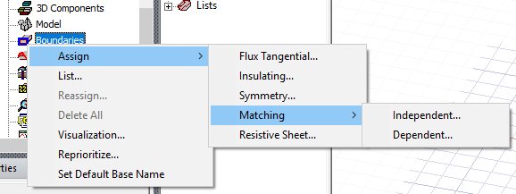
Boundaries supported are Flux Tangential, Insulating, Symmetry, Independent and Dependent Matching, and Resistive Sheet.
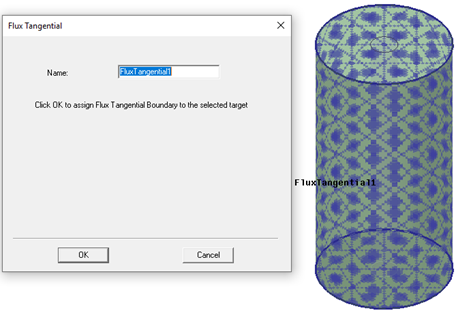
Flux Tangential boundaries can only be applied to face objects. Unlike the T-Omega formulation, the Neumann boundary condition on external faces is flux normal for A-Phi formulation. That is why a Flux Tangential boundary condition must be assigned when the magnetic field is tangential to the face.
-
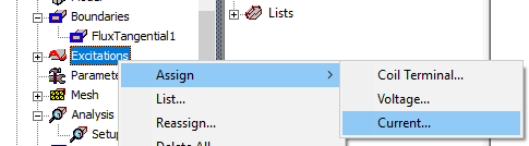
Excitations supported are winding (via Coil Terminal), voltage, and current. Winding excitation is assigned as in the Transient solver (Refer to Coil Terminals for more information on winding assignments). Voltage and Current excitations are also included on the Excitations > Assign menu:
Winding Excitations for A-Phi Formulation
Winding excitation is assigned as in the Transient solver (Refer to Assigning a Winding Setup for a Transient Solver for more information on winding assignments). For winding excitations, the coil terminals must be ordered according to the physical potential distribution. To do this:
- Right-click on the winding to open the context menu.
- Click on Order Coil Terminals to open the Order Coil Terminals dialog box.
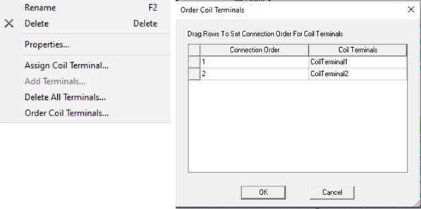
- Order the terminals by dragging them in the Order Coil Terminals dialog box.
Voltage Excitations for A-Phi Formulation
For designs with known potentials, select and assign a voltage excitation on each face.
You can also define initial currents for Voltage Excitation by checking the Initial Current box. When initial current is defined, the solver treats it as the current excitation. The default value is 0 A. You should select at least one voltage excitation without enabling the initial currents on a solid conduction path to set a reference potential. (If the path is touching the odd symmetry boundary, where the potential is set to 0 V, or if displacement effect is considered in the problem domain, then this rule does not apply on this path.)
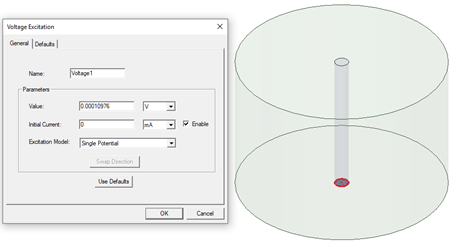
Voltage excitation supports three different excitation models:
-
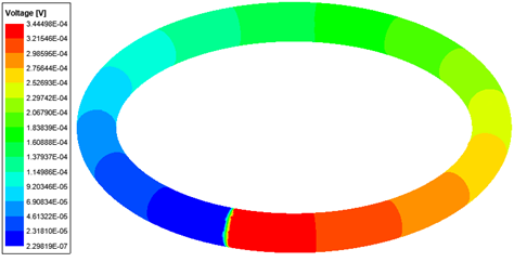
Single Potential: The solver treats the terminal as an equipotential terminal. Only one scalar electric potential DOF (Degree of Freedom) is assigned to the surface and the value of the DOF is set to the value that user inputs. This model must be used only at the external boundaries of the problem domain.
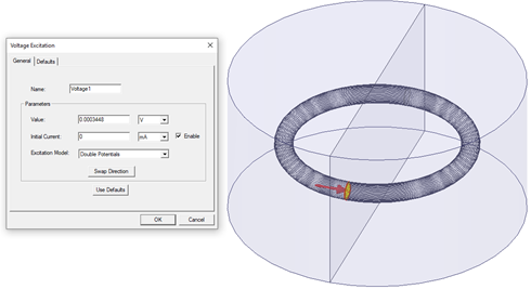
-
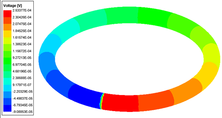
Double Potentials: The solver treats the terminal as a voltage (potential difference) terminal. At the terminal face, two scalar electric potential DOFs are defined and the DOFs are unknown. The difference between those potentials equals the voltage value that the user specified. If the voltage value is a positive quantity, higher potential is in the specified direction. This model must be used on faces inside the problem domain.
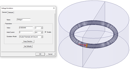
-
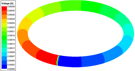
Double Potentials with Ground: The solver treats the terminal as voltage (potential difference) terminal. At the terminal face, two scalar electric potential DOFs are defined and both DOFs are known. The difference between those potentials equals to the voltage value that user specified. If the voltage value is a positive quantity, the DOF in the specified direction is set to the specified voltage value, and the DOF in the opposite direction is set to 0. This model must be used on faces inside the problem domain.
If the user does not define a reference potential on the same conduction path, the potentials at the terminal will be floating, so they are not unique. However, B, J, H, and all other quantities will be unique because they depend on the derivative of the potential.
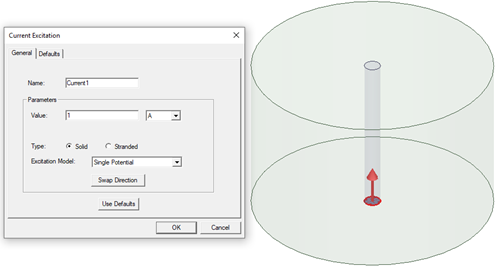
Current Excitations for A-Phi Formulation
For designs with known current values, the user selects and assigns a current excitation on each face. The user also selects the type of conductor: solid or stranded. Current excitation supports three different excitation models for a Solid conductor type based on how the potential DOF is assigned on the face:
- Single Potential: Only one scalar electric potential DOF is assigned to the surface and it is unknown. This model must be used only at the external boundaries of the problem domain.
- Double Potentials: At the terminal face, two electric scalar potential DOFs are defined and the DOFs are unknown. There is a potential difference at the terminal. The current will be unidirectional, and it will flow in the direction that user specifies if the current value entered is a positive quantity. This model must be used on faces inside the problem domain.
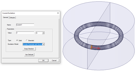
- Double Potentials with Ground: At the terminal face, two scalar electric potential DOFs are defined. The potential on the opposite side of the direction that user specified is set to 0. The current will be unidirectional, and it will flow in the specified direction if the current value entered is a positive quantity. This model must be used on faces inside the problem domain.
Rules/Limitations of Excitations on Conduction Paths
Winding Excitations
- One or two terminals can be defined on a conduction path: if the path is a loop, then only one coil terminal per coil must be defined, else only two coil terminals per coil must be defined (for both solid and stranded cases).
- More than two coil terminals are not allowed on a conduction path.
- Coil terminals must be ordered according to the physical potential distribution. One potential degree of freedom (DOF) is assigned to each external coil terminal. Two DOFs are assigned to each internal coil terminal. For windings with external coil terminals, there are two coil terminals defined for each conduction path. The potential DOF of the second terminal on a conduction path is linked to the potential DOF of the first terminal on the next conduction path, which means the coils are serially connected. That is why it is essential to create the coil terminals in the order of the actual potential distribution on serially connected coils (conduction paths). The potential on the last Coil Terminal is set to zero. The same rule for linking the DOFs applies to the windings with internal coil terminals.
Current Excitations
- For stranded current excitation: More than two terminals are not allowed on a conduction path. For a loop conduction path, one terminal is defined. For other conduction paths, user must define two terminals (in and out). A voltage terminal and a stranded current terminal cannot be defined on the same conduction path.
- For solid current excitations: At least one voltage excitation is to be defined as a reference potential on the same conduction path of the current excitation. If a current excitation with Double Potentials with Ground exists in the path, or displacement current is enabled, this requirement does not apply. Multiple current excitations on a conduction path are allowed.
Voltage Excitations
- There must be at least one voltage excitation on a conduction path with current/voltage excitations if displacement effect is not enabled (if the path is not touching the odd symmetry boundary, or there is no current/voltage excitation with Double Potentials with Ground excitation, where the potential is set to 0 V).
- Winding excitation cannot be defined together with voltage or current excitations on the same path.
- On a conduction path there can be multiple solid voltage and current terminals defined.
Independent/Dependent and Odd Symmetry Boundaries
- Excitations cannot be defined on Independent/Dependent boundaries.
- If a conduction path crosses an Odd Symmetry boundary, excitations must be defined at External boundaries because the default electric potential value is zero on the Odd Symmetry boundary. Voltage excitation can be used to set a different potential value on the face intersecting with an Odd Symmetry boundary. Also, any excitation (Coil Terminal, Voltage, or Current Excitation) assignment is allowed on the face intersecting with an Odd Symmetry boundary.
- If a conduction path crosses both Odd Symmetry and Independent/Dependent boundaries, the software's validation process does not allow one external terminal definition on the path. The user can select Perform minimal validations under Design Settings to simulate such designs at the user's own risk. Full model simulation is highly recommended for such designs.
Matrix Setup
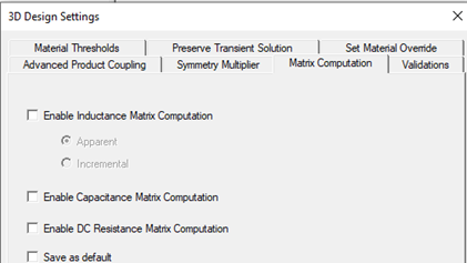
Parametric matrix setup is supported for the A-Phi transient solver. The user can define only one matrix setup for inductance, capacitance, or DC resistance calculations. For computation of the defined matrix, the user must select Enable Inductance Matrix Computation, Enable Capacitance Matrix Computation, or Enable DC Resistance Matrix Computation in the 3D Design Settings window:
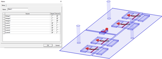
The user selects signals and grounds for the matrix of interest. For the inductance matrix, the followings are restrictions on ground selections:
- Ground selection is not allowed for windings, because they are internally grounded.
- Ground selection is not allowed for stranded current excitations since no potential is defined on the conduction path.
- Ground selection is not allowed for current excitations with double potentials and double potentials with ground.
- Ground selection is only available for Voltage excitation with Single Potential model. Ground selection is not allowed for voltage excitations with double potentials and double potentials with ground.
It is highly recommended that ground selection be as in the nominal problem setup, especially for designs with multi-terminal excitations on a conduction path. Other solver types do the matrix computation after the solution of nominal problem so it is fully post-processed, and the user can select different signal/ground/return path configurations. However, the transient solver is computing the matrix at each timestep and the computation is highly dependent on how the current flows on a path, especially for designs with multiple excitations on the path.
The capacitance matrix is computed using the electrostatic energy stored in a system under 1 V excitation for one selected signal and 0 V for all others. Based on the selection of signals and grounds, the solver computes the capacitance matrix of the system. Stranded conductors and floating conductors (no signal or ground assigned) are treated as equipotential surfaces. For the capacitance matrix, the following rule applies for the ground selection:
- There must be at least one ground selection in the Matrix setup if there is no internal zero reference potential defined in the design. Odd Symmetry, winding excitation, and double potentials with ground excitation model are examples of internal grounds.
The resistance matrix is computed with the assumption of a DC conduction solution using the material values at time zero, so it is time independent. For stranded conductors, the solver internally calculates the stranded resistance values. The resistance value (the user typically inputs the stranded resistance value in addition to the source resistance) in the winding excitation setup is not included in the DC resistance matrix.
Postprocessing Support
The A-Phi transient solver supports all the postprocessing features of the transient solver. Additionally, the following features are supported:
- Voltage in the Field Plot and in the Fields Calculator; there are cases where no voltage is defined in an object (in a stranded object, or in an object with no eddy or displacement effect setting).
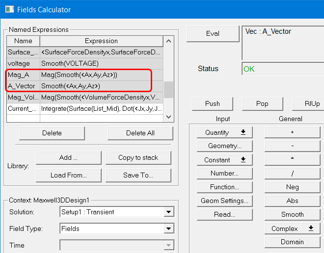
- Magnetic vector potential in the Fields Calculator:
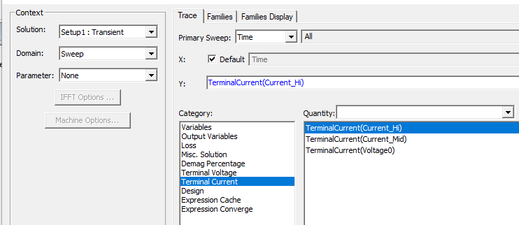
- Voltage and current quantities at the Voltage and Current Terminals; the current computed at any terminal is assumed to be flowing into the problem domain.
3D Layout Component
With the A-Phi transient solver, Maxwell 3D can run a transient solution that includes a 3D layout component. This feature makes it easier to simulate electronic applications such as multilayer PCBs to calculate the Lorentz force due to trace currents and external magnetic fields.
Running a transient solution on a design with a 3D layout component requires the use of both HFSS 3D Layout and Maxwell 3D products. You first create the layout component with excitations, mesh operations and RLC components defined in HFSS 3D Layout. Then, you must import the component in a Maxwell 3D design. Maxwell will automatically import the layout excitations and circuit components (RLC). You need to select the type of the excitations (voltage or current), and enter certain information related to each excitation type. The rest of this section will explain the details of the entire design flow of a Maxwell design with the 3D layout component.
Creating a Layout Component in HFSS 3D Layout
You can either create a component from scratch or can import a third party layout design data (Refer to Importing Layout Design Data in the HFSS 3D Layout help). You can use all capabilities of the Layout Editor such as geometry check, shorts/opens in a design.
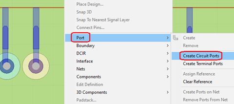
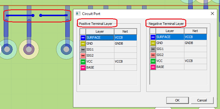
You need to define excitations in the Layout design by creating circuit ports. Existing port definitions are still valid ( refer to Circuit Ports and Elements in the HFSS 3D Layout Help). In the Layout Editor, one way to create a circuit port is to right-click the geometry view, select Port > Create Circuit Ports, select two points, and then select a Positive Terminal Layer and Negative Terminal Layer in the pop-up dialog.
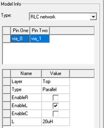
You can add lumped circuit elements into the design. For RLC support, you define a component for each lumped element (R, L, or C). The component has two pins and associated padstacks. Each component must have only one lumped element type (user must enable only one as shown). Note that serial or parallel connection of RLC is not supported so Maxwell will ignore the Type selection.
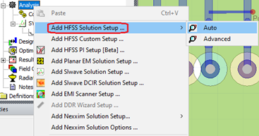
Mesh operations for the layout design should be defined in the Layout. To assign mesh operations, first add an HFSS solution setup. Then right-click the solution setup and select Assign Mesh Operation:
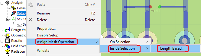
In the Select Geometry dialog, you can specify the Max Length to refine the mesh. Note that the solution setup is not used for the solution of the design.

Once the design is complete, you can save it as a component or just save the layout design. When the component is imported in Maxwell, the design data including layout model (with virtual geometry view), excitation assignments, mesh operations, RLC data, and materials will be automatically imported into Maxwell. Pin groups are imported as excitations, but the pin group information is still available for simulation.
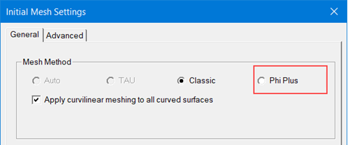
For a Maxwell design with a 3D layout component, the Phi Plus mesher setting is available in the Maxwell 3D > Mesh > Initial Mesh Settings dialog box; it replaces the TAU mesher, which will be grayed out.
Layout Component Features in Maxwell 3D
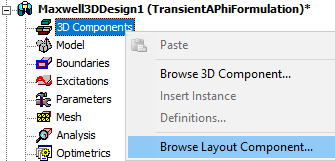
To import a layout design as component, right-click 3D Components, select Browse Layout Component...
In the Create Layout Component dialog, there are two options to import:
- Import .aedbcomp file; the .aedbcomp file should be a non-encrypted layout component, otherwise there will be an error message preventing such import.
- Browse to project aedb folder to import a layout design.

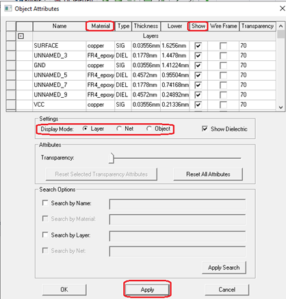
To view object attributes, click Object Attributes in the component property window.
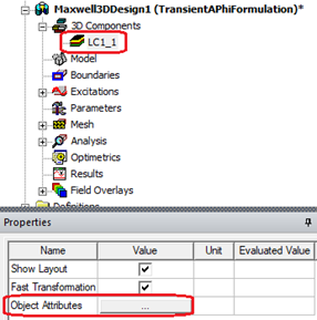
In the Object Attributes dialog, you can view object attributes such as: Name, Material, Type, and so on. There are different display modes: Layer, Net, and Object. In the Show column, after changing the object visibility, you can see the checked objects in the geometry view by clicking Apply button.
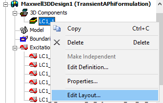
You can modify the Layout component. To edit the layout, right-click on the component, and select Edit Layout... This will open the layout design of the component in a new project. You can then modify the design in the new project. Once the modified design is saved, Maxwell will automatically update the layout component.
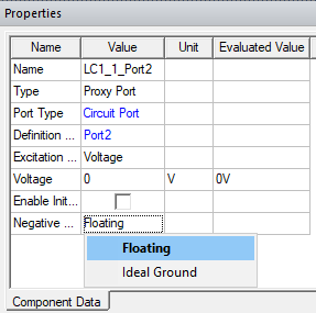
After a layout design is imported into Maxwell, the layout circuit port will be converted into a Proxy Port in Maxwell. Each proxy port has two nodes. One node is positive (current flows into the conductor), and the other one is negative (current flows out of the conductor). A node can be a terminal or a pin group (group of terminals). All terminals of a pin group are parallel connected, so they have the same potential value. Maxwell treats a terminal as an equipotential surface. Examples of port definitions are shown below:

The Excitation Type can be Voltage or Current.
- For voltage excitation, enter a voltage value and select the behavior of the negative terminal (Ideal Ground or Floating). The default is Floating. The solver applies the specified voltage value as a potential drop between the terminals. If Ideal Ground is selected, the negative terminal potential is set to 0 V. For Floating, the negative terminal potential is unknown. You can also specify the initial current value by selecting Enable Initial Current.
- For current excitation, enter a current value and select the behavior of the negative terminal.
You can continue to use existing mesh operations for non-component objects. The suggested mesh method is A-Phi for a layout component. You can specify this in the Maxwell Initial Mesh Settings.
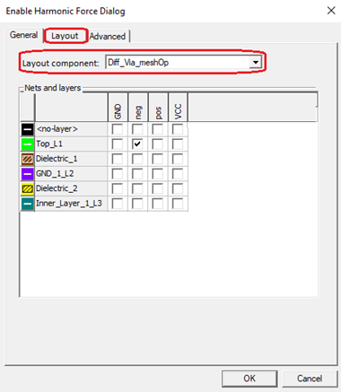
To calculate harmonic force on objects, right-click the design, then select Enable Harmonic Force Calculation...
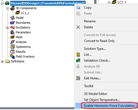
In the Enable Harmonic Force Dialog, on the Layout tab, you can select one layout component from the Layout component drop-down menu, and select <layer, net> pairs in the following grid, each <layer, net> pair represents the object(s) in the intersection of corresponding layer and net.
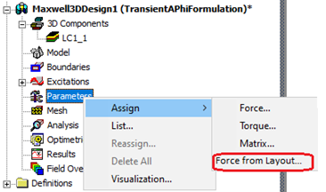
To calculate Lorentz force on objects, right-click Parameters, and select Assign > Force from Layout... Note that this menu item will only show up if there is a layout component.
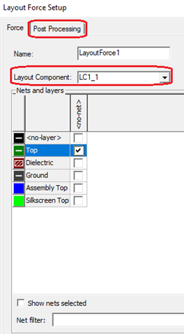
In the Layout Force Setup dialog, on the Force tab, select one layout component from the Layout Component drop-down menu, and select <layer, net> pairs in the following grid. Each <layer, net> pair represents the object(s) in the intersection of corresponding layer and net. Then, select the post-processing coordinate system on the Post-Processing tab.
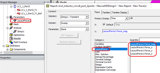
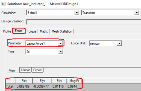
The LayoutForce can be plotted from the reporter as shown below:
Layout force can also be viewed in the Solution Data Dialog.
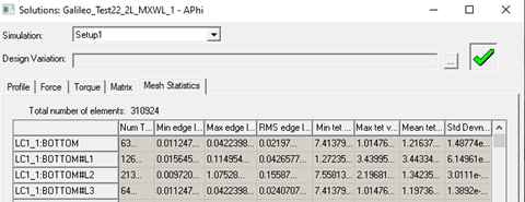
Mesh Statistics for layout objects can also be viewed in the Solutions window:
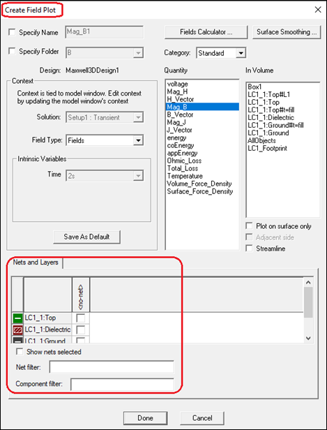
To review results from the Field reporter, you can select the layout objects in the Create Field Plot dialog box:
Limitations for the 3D Layout Component Feature
- Field calculator for expression cache/output variables can only be setup after solving.
- Conduction path functionality in Maxwell is not applicable to layout component.
Related Topics
Technical Notes: A-Phi Formulation in Maxwell 3D (Transient)
Transient A-Phi Formulation Boundaries and Excitations
Transient A-Phi Formulation Boundary Conditions
Transient A-Phi Formulation Excitations