


VM-LSDYNA-SOLVE-050
VM-LSDYNA-SOLVE-050
Lateral Vibration of a Rectangular Plate
Overview
| Reference: | Timoshenko, S., & Young, D. H. (1971). Vibration problems in engineering (3rd ed.). D. Van Nostrand Co., Inc., p.338, article 53. |
| Analysis Type(s): | Implicit Vibration Analysis |
| Element Type(s): |
2D Quadrilateral Shell Elements 3D Hexahedral Solid Elements |
| Input Files: | Link to Input Files Download Page |
Test Case
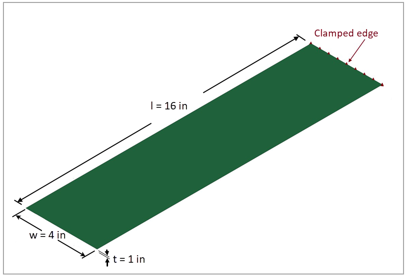
This test case models the lateral vibration of a rectangular plate with one smaller edge subjected to a clamped condition. The objective is to validate the first natural frequency of lateral vibration of the structure. The rectangular plate has a length of 16 in, a width of 4 in, and a thickness of 1 in. The test case is implemented in LS-DYNA using two different element types (2D shells and 3D solids). Figure 174 illustrates the domain dimensions and boundary conditions.
This problem is also presented in test case VM66 in the Mechanical APDL Verification Manual.
The following table lists the material and geometric properties of the test case.
| Material Properties | Geometric Properties |
|---|---|
|
Young's modulus (E) = 3 ⋅10 7 Pa Poisson’s ratio (ν) = 0.3 Density (ρ) = 7.28 ⋅ 10 -4 lbf-s2/in4 |
Length (l) = 16 in Width (w) = 4 in Thickness (t) = 1 in |
Analysis Assumptions and Modeling Notes
The natural frequency  of lateral vibration of the plate can be calculated as:
 | (24) |
where
 is a dimensionless parameter is a dimensionless parameter |
 is the plate length is the plate length |
 is the Young’s modulus is the Young’s modulus |
 is the moment of inertia is the moment of inertia |
 is the material density is the material density |
and  is the cross-section area is the cross-section area |
The parameter is a function of the
mode index  and the boundary conditions. For the condition of one clamped edge, the
dimensionless parameter = 1.875. The moment of
inertia of the cross-section is
and the boundary conditions. For the condition of one clamped edge, the
dimensionless parameter = 1.875. The moment of
inertia of the cross-section is  , where
  is the width and
  is the thickness. Therefore, the natural frequency for the first lateral
vibration mode is 128.08 Hz.
is the thickness. Therefore, the natural frequency for the first lateral
vibration mode is 128.08 Hz.
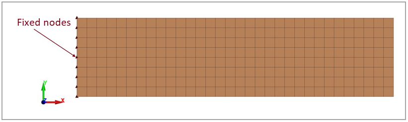
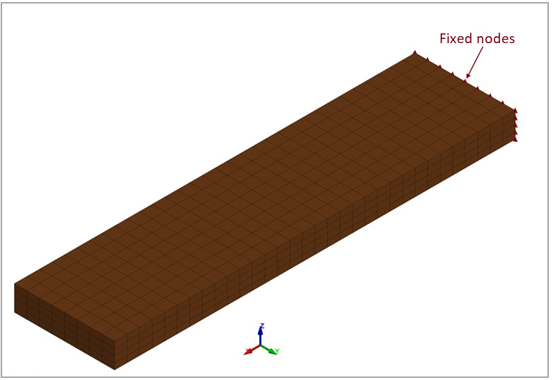
One part is defined to represent the rectangular plate, using a linear elastic material card (*MAT_ELASTIC) with properties shown in the above table. The 2D plate model is meshed with 2D quadrilateral shell elements and uses a fully integrated shell formulation with higher accuracy (ELFORM=–16). The 3D plate model is meshed with 3D hexahedral solid elements and uses a nine-point enhanced strain solid element formulation (ELFORM=18). The nodes corresponding to the clamped segments of the plate are grouped using *SET_NODE_LIST, and the keyword *BOUNDARY_SPC_SET is used to define the constraint of this node set (translational and rotational constraint about the three axes). The keywords *CONTROL_IMPLICIT_GENERAL (IMFLAG=1), *CONTROL_IMPLICIT_DYNAMICS (IMASS=0), and *CONTROL_IMPLICIT_EIGENVALUE (NEIG=1) are used to activate the implicit eigenvalue static analysis with one eigenvalue to be extracted.
Results Comparison
The visualization of the first lateral mode can be performed by reading the d3eigv file generated for the modal analysis. To quantify the error between the theoretical and LS-DYNA results, the first natural frequency of the lateral vibration of the plate and their relative errors are calculated and shown in the following table for both element types. This comparison verifies the agreement between the natural frequencies.
The table below compares the natural frequencies for the first natural frequency of the lateral vibration of the plate calculated using the modal theory and the LS-DYNA model
| Results | Target | LS-DYNA Solver | Error (%) |
|---|---|---|---|
|
Natural Frequency (Hz) 2D Shell Elements | 128.08 | 127.87 | -0.17% |
|
Natural Frequency (Hz) 3D Solid Elements | 128.08 | 127.74 | -0.27% |