VM-LSDYNA-SOLVE-040
VM-LSDYNA-SOLVE-040
Buckling of a Stepped Rod
Overview
| Reference: | Young, W. C. & Budynas, R. G. (2002). Roark's formulas for stress and strain (7th ed.). McGraw-Hill, p.720, table 15.1, case 2a. |
| Analysis Type(s): | Implicit Eigenvalue Buckling Analysis |
| Element Type(s): | Linear Elastic Material Model |
| Input Files: | Link to Input Files Download Page |
Test Case
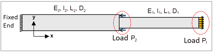
This finite element (FE) simulation investigates the elastic buckling behavior of a stepped cantilever rod subjected to two axial loads: a tensile force P1 and a compressive force P2. The applied loads induce tension in the thinner section of the rod (Rod 1), and compression in the thicker section (Rod 2), as illustrated schematically in Figure 145. The LS-DYNA eigenvalue buckling analysis (with the main keywords *CONTROL_IMPLICIT_BUCKLE and *CONTROL_IMPLICIT_GENERAL) is employed to predict the critical load multiplier associated with the first buckling mode in the compressed, thicker segment of the rod. The simulation result is validated against Roark's empirical buckling formula, which is fundamentally based on Euler's classical buckling theory, showing excellent agreement between the numerical and analytical solutions.
For this study, both rod sections are modeled as linear elastic components with different diameters (D1 = 10 mm and D2 = 11.982 mm) and lengths (L1 = 100 mm and L2 = 200 mm). The right (free) end of the rod is subjected to a tensile load of 1000 N while a compressive load of 2000 N is applied at the annular step. This case serves as a reference to verify the accuracy and reliability of the LS-DYNA eigen solver.
The table below shows the geometric properties, material properties, as well as loading and boundary conditions.
| Material Properties | Geometric Properties | Loading |
|---|---|---|
|
Density ρ = 7850 kg/m3 Young's modulus E = 2.0E+11 Pa Poisson's ratio ν = 0.30 |
Diameter D1 = 0.010 m Diameter D2 = 0.011982 m Length L1 = 0.100 m Length L2 = 0.200 m |
Tensile force at free end P1 = 1000 N Compressive force at annular step P2 = –2000 N |
As illustrated in Figure 145, the axial loads in the LS-DYNA simulation are applied using equal nodal point loads—that is, the total force is distributed evenly across the nodes on the relevant cross sections. This is implemented using the *LOAD_NODE_SET keyword. To ensure an approximately uniform load distribution, it is important that the nodes on the loaded surfaces are spaced relatively evenly. Another option is to apply the axial loads as uniformly distributed tensile and compressive pressure loads over the cross-sectional areas.
For the first buckling mode in the present scenario, Roark provides an empirical equation,
which is fundamentally derived from Euler's classical buckling theory. Roark's equation
predicts the critical axial compressive force in the thicker rod,  , as follows:
 | (8) |
where  is the Young's modulus of the material, and
  is the area moment of inertia of the cross-section. In this equation,
 is an empirical factor that depends on three key ratios of
  ,
,  , and
, and  . For the present case study, these ratios are
  ,
,  , and
, and  . Based on these values, the empirical constant is
  . Consequently, the load multiplier corresponding to the first buckling mode
is expected to be
. Consequently, the load multiplier corresponding to the first buckling mode
is expected to be  as calculated using the following equation:
 | (9) |
Analysis Assumptions and Modeling Notes
The deformable rods are modeled using the *MAT_001/*MAT_ELASTIC material model in the LS-DYNA application, representing linear elastic behavior with properties typical of structural steel. Both rods, integrated into the same part, are assigned a density of 7850 kg/m³, a Young's modulus of 2.0E+11 Pa, and a Poisson's ratio of 0.3. As shown in Figure 146, the entire geometry is discretized using a combination of hexahedral and tetrahedral solid elements (ELFORM = 1). A finer mesh is applied near the small annular step region to improve accuracy and ensure a more uniform application of the compressive load. Hourglass control is applied using Type 6 (Belytschko–Bindeman formulation), a stiffness-based method effective for solid elements. The hourglass coefficient QM = 0.1 is used which scales the artificial stiffness added to suppress zero-energy hourglass deformation modes. The left end of the stepped rod is fully fixed, with all translational and rotational degrees of freedom constrained to eliminate rigid body motion. The simulation is performed using the SI unit system (N, m, kg, s), though it can be readily adapted to other consistent unit systems if required.

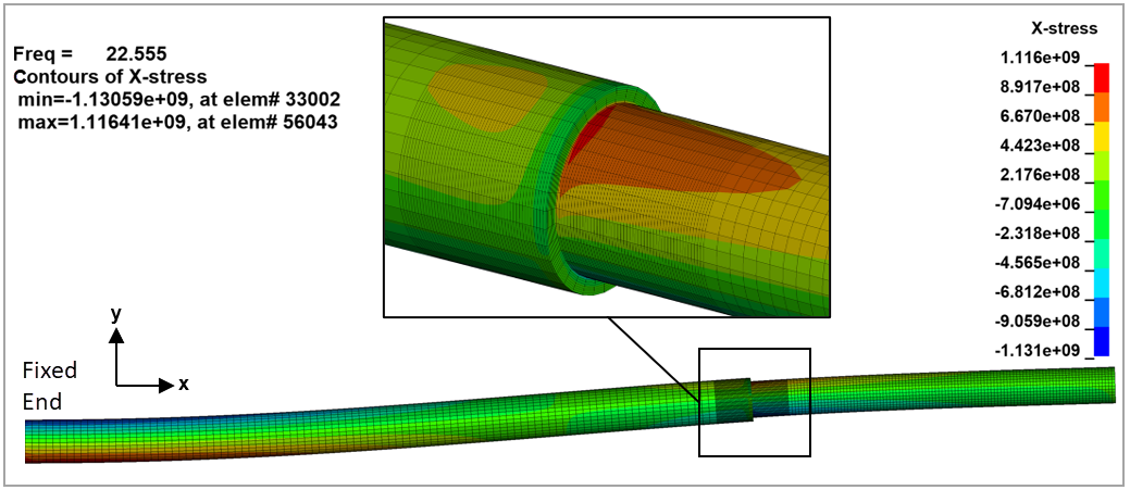
In general, using the Massively Parallel Processing (MPP) version of LS-DYNA for eigenvalue buckling simulations is recommended. The buckling load factors (eigenvalues) are printed in the eigout file. These eigenvalues represent multipliers to the applied loads that produce the corresponding buckling loads. Therefore, the critical buckling load can be determined by multiplying the applied load by the appropriate eigenvalue. Pay attention to the sign, positive or negative, of the written eigenvalues. The associated buckling mode shapes are stored in the d3eigv output file. For the buckling analysis, the first positive eigenvalue corresponds to the onset of compressive buckling, while negative values may indicate tension or non-physical modes in systems with mixed loading. To include stress output in the d3eigv files, the keyword *CONTROL_IMPLICIT_EIGENVALUE should be defined with NEIG = 0 and MSTRES = 1. This ensures that stresses are computed for the eigenmodes and included in the generated d3eigv file.
Results Comparison
To verify the accuracy of the simulation and the LS-DYNA eigenvalue buckling solver, the predicted value of the target parameter is compared against the empirical equation provided by Roark. In this case, the target is the first positive eigenvalue written in the eigout file which represents the load multiplier associated with the first compressive buckling mode. As shown in the results table below, the simulation captures this critical buckling load multiplier with high accuracy, showing a deviation of only 0.27% from the theoretical value.
The results table below shows the value of the load multiplier for the first buckling mode versus the analytical solution.
| Results | Target | LS-DYNA Solver | Error (%) |
|---|---|---|---|
| Load Multiplier | 22.50 | 22.56 | 0.27 |
Figure 147 shows the predicted first buckling mode shape and corresponding axial stress (X-stress) distribution. Notice the plot displays the amplified deformation (displacement factor = 3).