VM-LSDYNA-SOLVE-041
VM-LSDYNA-SOLVE-041
Buckling of a Curved Panel
Overview
| Reference: | Young, W. C., & Budynas, R. G. (2002). Roark's formulas for stress and strain (7th ed.). McGraw-Hill, p.737, table 15.2, case 21b. |
| Analysis Type(s): | Implicit Eigenvalue Buckling Analysis |
| Element Type(s): | Linear Elastic Material Model |
| Input Files: | Link to Input Files Download Page |
Test Case
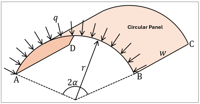
The present finite element (FE) simulation investigates the elastic buckling behavior of a curved panel under a uniform radial pressure of q = 1 MPa. The analysis uses the LS-DYNA eigenvalue buckling solver using the main keywords *CONTROL_IMPLICIT_BUCKLE and *CONTROL_IMPLICIT_GENERAL to determine the critical load multiplier corresponding to the panel's first buckling mode. The numerical results are validated against Roark's analytical buckling formula, showing excellent agreement between the two approaches.
The simulation setup is schematically illustrated in Figure 148. The panel is modeled as a linear elastic shell with a uniform thickness of t = 5 mm, a radius of curvature r = 50 mm, a central angle of 2α = 120°, and a width of w = 30 mm. The curved edges (AB and CD) are free, while the straight edges (BC and AD) are fixed. This case serves as a reference to verify the accuracy and reliability of the LS-DYNA eigenvalue buckling solver.
The table below shows the geometric properties, material properties, as well as the loading and boundary conditions.
| Material Properties | Geometric Properties | Loading |
|---|---|---|
|
Density ρ= 0.007850 g/mm3 Young's modulus E = 2.0E+5 MPa Poisson's ratio ν = 0.30 |
Radius of curvature r = 50 mm Uniform thickness t = 5 mm Central angle 2α = 120° Width w = 30 mm |
Uniform radial pressure q = 1 Mpa Free curved edges Fixed straights edges |
For the first buckling mode in the current scenario, Roark's predictive equation for the
critical radial pressure  is as follows:
 | (10) |
where  is the Young's modulus of the material, and
  is an empirical factor that depends on 𝛂, half of the central angle.
For the present case, = 4.37. Consequently, the load multiplier corresponding to the first
buckling mode is expected to be 𝛌= 331.45, as calculated using the following
equation:
is an empirical factor that depends on 𝛂, half of the central angle.
For the present case, = 4.37. Consequently, the load multiplier corresponding to the first
buckling mode is expected to be 𝛌= 331.45, as calculated using the following
equation:
 | (11) |
Analysis Assumptions and Modeling Notes
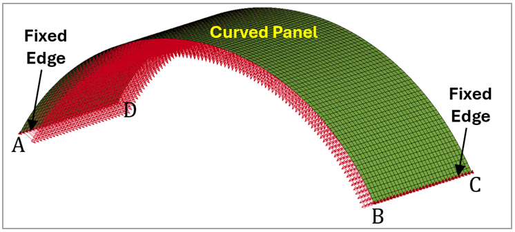
The deformable panel is modeled using the *MAT_001/*MAT_ELASTIC material model in LS-DYNA, representing linear elastic behavior with properties typical of structural steel. Specifically, the material is assigned a density of 7850 kg/m³, a Young's modulus of 2.0E+11 Pa, and a Poisson's ratio of 0.3. As shown in Figure 149, the entire geometry is discretized using quadrilateral shell elements. Fully integrated shell elements with higher accuracy (ELFORM = -16) are employed, eliminating the need for hourglass control. The straight edges of the panel are fully constrained, with all translational and rotational degrees of freedom fixed. The simulation is conducted using a non-SI unit system (g, mm, ms, N, MPa), though it can be readily adapted to other consistent unit systems if required.
In general, using the Massively Parallel Processing (MPP) version of LS-DYNA for eigenvalue buckling simulations is recommended. The buckling load factors (eigenvalues) are printed in the eigout file. These eigenvalues represent multipliers to the applied pressure that produce the corresponding buckling pressure. Therefore, the critical buckling pressure can be determined by multiplying the applied pressure by the appropriate eigenvalue. The associated buckling mode shapes are stored in the d3eigv output file. For buckling analysis, the first positive eigenvalue corresponds to the onset of compressive buckling, while negative values may indicate tension or non-physical modes in systems with mixed loading. To include stress output in the d3eigv files, the keyword *CONTROL_IMPLICIT_EIGENVALUE should be defined with NEIG = 0 and MSTRES = 1. This ensures that stresses are computed for the eigenmodes and included in the generated d3eigv file.
Results Comparison
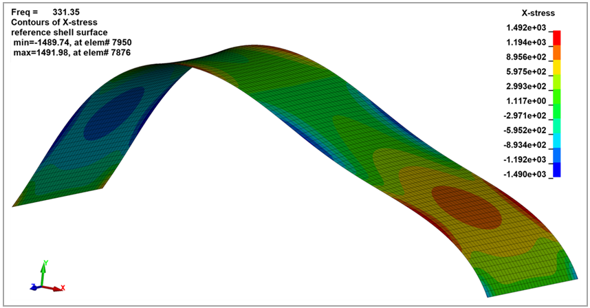
To verify the accuracy of the simulation and the reliability of the LS-DYNA eigenvalue buckling solver, the predicted value of the target parameter is compared against the analytical solution provided by Roark. In this case, the target is the first positive eigenvalue recorded in the eigout file, which represents the load multiplier associated with the first compressive buckling mode. As summarized in the results table below, the simulation accurately predicts this critical buckling load multiplier, with a deviation of only −0.03% from the expected value. Figure 150 shows the predicted first buckling mode shape along with the corresponding X-stress distribution.
| Results | Target | LS-DYNA Solver | Error (%) |
|---|---|---|---|
| Load Multiplier | 331.45 | 331.35 | -0.03 |