VM-LSDYNA-SOLVE-039
VM-LSDYNA-SOLVE-039
Buckling of a Uniform Rod
Overview
| Reference: | Timoshenko, S. P., & Gere, J. M. (2009). Theory of elastic stability (2nd ed., Dover ed.). Dover Publications. |
| Analysis Type(s): | Implicit Eigenvalue Buckling Analysis |
| Element Type(s): | 3D Solid Mesh with Hexahedral Elements |
| Input Files: | Link to Input Files Download Page |
Test Case
The finite element simulation presented in this test case models the elastic buckling behavior of a uniform cantilever rod under axial compressive loading. Employing the LS-DYNA eigenvalue buckling analysis with the main keywords *CONTROL_IMPLICIT_BUCKLE and *CONTROL_IMPLICIT_GENERAL, the simulation predicts the critical load multiplier corresponding to the lowest-energy deformation the rod takes when it begins to buckle, known as the first buckling mode.
The resulting load multiplier is validated against Euler’s classical buckling formula to verify the accuracy of the LS-DYNA eigen solver. This comparison demonstrates the accuracy of the simulation and suggests the analysis may serve as a model for cases involving more complex geometries, such as stepped rods (see VM-LSDYNA-SOLVE-040 in the Ansys LS-DYNA Verification Manual).
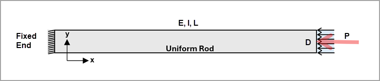
Figure 142 displays the case's uniform rod modeled as a linear elastic structure fixed at one end and compressed at the free end. The table that follows shows the material and geometric properties as well as the loading conditions that define the case.
| Material Properties | Geometric Properties | Loading |
|---|---|---|
|
Density = 7850 kg/m3 Young's modulus = 2.0E+11 Pa Poisson's ratio = 0.3 |
Diameter D = 0.1 m Length L = 2 m |
Compression force at free end = 10 kN or Pressure at free end = 1273239.54 Pa |
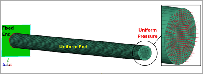
This simulation applies an axial load with uniform pressure distribution. Alternatively, you may apply the axial load by distributing the total force across nodes at the free end. In this approach, you should space nodes equally to provide an approximate uniform distribution of force.
To validate the simulation, Euler’s classical buckling theory serves as a reliable benchmark and provides a fundamental analytical approach for estimating the critical axial force at which a slender, elastic column becomes unstable and buckles in idealized conditions.
For the first buckling mode, the critical load is calculated using the following equation:
 | (6) |
Where:
 represents the critical buckling load represents the critical buckling load |
 represents the Young's modulus of the material represents the Young's modulus of the material |
 represents the area moment of inertia of the cross section represents the area moment of inertia of the cross section |
 represents the effective length factor, which depends on the boundary conditions represents the effective length factor, which depends on the boundary conditions |
 represents the unsupported length of the column represents the unsupported length of the column |
Equation 6 (above) assumes linear elasticity, small deformations, and a perfectly straight, slender column without initial imperfections.
The effective length factor in this test case is  =2, with one end of the rod fixed and the other free. Using Equation 7 (below), where
  represents the applied axial load (
 =10 kN), the expected load multiplier for the first buckling mode is
  = 60.56.
 | (7) |
Analysis Assumptions and Modeling Notes
The deformable rod is modeled using *MAT_001/*MAT_ELASTIC, representing a linear elastic material with properties typical of structural steel (see the Test Case Description for exact material properties). The rod is fixed at the left end, where all translational and rotational degrees of freedom are constrained to eliminate rigid body motion.
In this model, the entire geometry is discretized using hexahedral solid elements (ELFORM=1). Hourglass control is applied using Type 6 (Belytschko–Bindeman formulation), a stiffness-based method effective for solid elements. The default hourglass coefficient QM = 1.0 is used, a coefficient that scales the artificial stiffness added to suppress zero-energy hourglass deformation modes.
The simulation uses the SI unit system (N, m, kg, s), but you may adapt the simulation to other systems as needed.
Using the Massively Parallel Processing (MPP) version of LS-DYNA for eigenvalue buckling simulations is recommended. Buckling load factors (eigenvalues) are printed in the eigout file. These eigenvalues represent multipliers to the applied loads that produce the corresponding buckling loads. Therefore, the critical buckling load can be determined by multiplying the applied load by the appropriate eigenvalue.
Note whether eigenvalues are positive or negative. For buckling analysis, the first positive eigenvalue corresponds to the onset of compressive buckling, while negative values may indicate tension or non-physical modes in systems with mixed loading.
The associated buckling mode shapes are stored in the d3eigv output file. To include stress output in the d3eigv files, define the keyword *CONTROL_IMPLICIT_EIGENVALUE with NEIG = 0 and MSTRES = 1. This ensures that stresses are computed for the eigenmodes and included in the generated d3eigv file.
Results Comparison
The table below demonstrates that the simulation accurately predicts the load multiplier of the first buckling mode, validating the accuracy of the LS-DYNA eigen solver.
| Results | Target | LS-DYNA Solver | Error (%) |
|---|---|---|---|
| Load Multiplier | 60.56 | 60.39 | -0.28 |
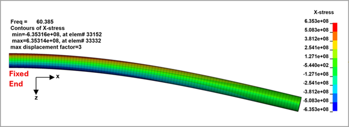
Figure 144 shows the predicted buckling mode shape, corresponding axial stress (X-stress) distribution, and amplified deformation (displacement factor = 3).