VM-LSDYNA-SOLVE-038
VM-LSDYNA-SOLVE-038
Rectangular Plate with Circular Hole Subjected to Tensile
Loading
Overview
| Reference: | Budynas, R. G., & Nisbett, J. K. (2015). Shigley’s Mechanical Engineering Design (10th ed.). New York, NY: McGraw-Hill Education. (p.125, figure 3-29; p.1034, figure A-15-1.) |
| Analysis Type(s): | Linear Static Structural Analysis – Implicit and Explicit with Damping |
| Element Type(s): |
10-Node Tetrahedral Solid Elements |
| Input Files: | Link to Input Files Download Page |
Test Case
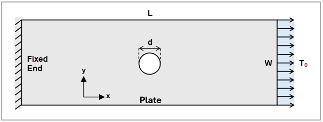
The simulation models a 3D rectangular plate with a central circular hole, a geometric irregularity, subjected to linear static structural analysis to evaluate stress concentration effects. The left end of the plate is fully fixed, while a uniform tensile pressure is applied to the right end. The plate is modeled using 10-node tetrahedral elements with a finer mesh near the hole to capture stress gradients accurately. The schematic of the present test case is shown in Figure 136.
Figure 136: Schematic of the test case: a rectangular plate with circular hole subjected to tensile loading
The table below shows the geometric properties, material properties, as well as loading and boundary conditions. The material is assumed to be linear elastic and isotropic, obeying Hooke's Law. No plasticity, creep, thermal expansion, or failure criteria are included.
| Material Properties | Geometric Properties | Boundary Conditions and Loading |
|---|---|---|
|
*MAT_ELATIC (001) Young's modulus = 1E6 Pa Poisson's ratio = 0.48 Density = 1100 kg/m3 |
Length = 15 m Width = 5 m Thickness = 1 m Hole diameter = 1 m |
One fixed end One loaded end Uniform tensile pressure = -100 Pa System damping constant = 5 |
The primary output of interest is the maximum normal stress in the x-direction,
particularly near the hole where stress concentration is expected. The central circular hole
is a stress raiser. Using the theoretical stress concentration factor  , the actual maximum normal stress at the geometric discontinuity
 can be calculated from the nominal stress
  as
as
 | (3) |
where  depends only on geometry—the ratio of the hole diameter to the width
(
depends only on geometry—the ratio of the hole diameter to the width
( ). The nominal stress
  can be calculated using either
 | (4) |
| or |
 | (5) |
where  in Equation 4 is the applied
uniform tensile pressure, equal to 100 Pa in the present case, and
in Equation 4 is the applied
uniform tensile pressure, equal to 100 Pa in the present case, and
 and
and  represent the plate's dimensions. In Equation 5,
  denotes the applied force and
  is the plate thickness. For the present case,
  . Thus,
  (unitless) and
  . Consequently,
  .
.
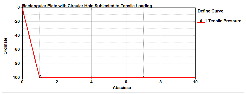
In both implicit and explicit time integration schemes, the spatially uniform tensile pressure was ramped up as shown in Figure 137.
Analysis Assumptions and Modeling Notes
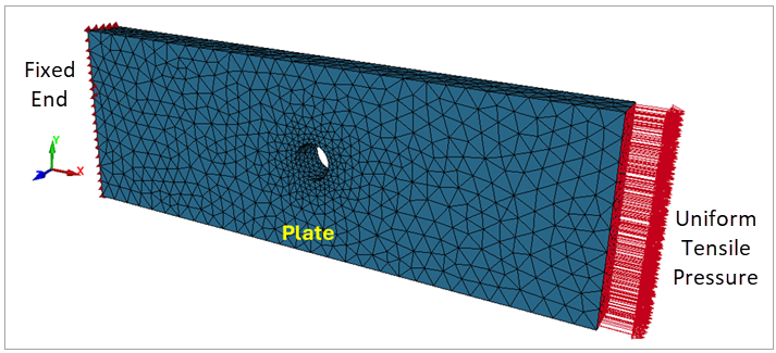
The entire domain is discretized using ten-node tetrahedral solid elements (ELFORM=16). A refined mesh near the hole is employed to capture stress gradients accurately near this geometric discontinuity which causes stress concentrations. One end of the plate is fully fixed, with all translational and rotational degrees of freedom constrained to prevent rigid body motion. A uniform tensile pressure is applied on the opposite end, normal to the surface, to represent a far-field uniaxial tensile load. No contact interfaces are defined since the model consists of a single continuous solid body. The simulation is conducted in the SI unit system (N, m, kg, s) but could be adapted to other consistent unit systems as needed.
Figure 138: Model setup for 3D rectangular plate with a central circular hole subjected to tensile pressure
Results Comparison
To verify the accuracy of the simulation, the predicted values of the target parameter—that is, the maximum normal stress in the x direction—were compared against the theoretical values calculated with the stress concentration factor. As shown in the results table below, the implicit and explicit solvers predicted the target stress within -0.11% and -0.07%, respectively, of the theoretical values, validating the numerical results. The maximum normal stress is shown in Figure 139, while Figure 140 shows the amplified deformation of the plate at six seconds. Notably, in both time integration schemes, oscillations were observed at the free end prior to the application of global damping.
| Results | Target | LS-DYNA Solver | Error (%) |
|---|---|---|---|
| Max. Normal X Stress | 312.5 | 312.29 (explicit) | –0.07% |
| Max. Normal X Stress | 312.5 | 312.15 (implicit) | –0.11% |
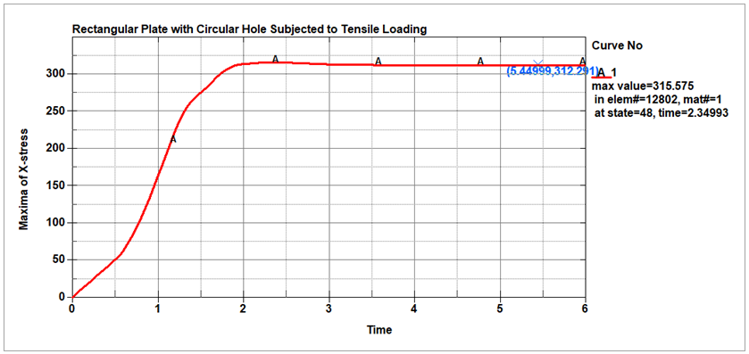
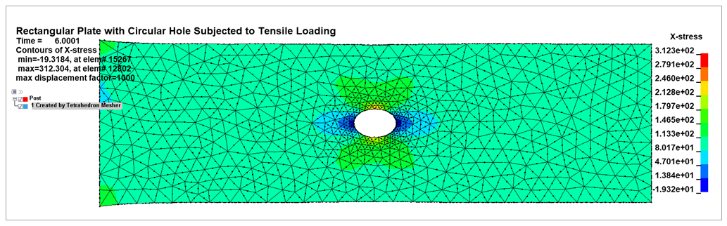
Figure 140: Contours of maximum normal stress in the x direction (Pa) with deformations amplified for better visualization in the explicit modeling
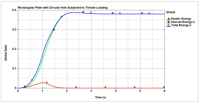
As the energy plots in Figure 141 indicate, the simulation is stable. The kinetic energy (red curve) peaks early, then drops to near zero, proving that the system reaches a quasi-static state. Internal energy (green curve) increases steadily and plateaus as loading finishes. This is strain energy stored in the plate due to tension. Total energy (blue curve) matches the internal energy closely after time ≈ 2 s, indicating minimal artificial energy input. Thus, the result is dominated by strain energy.
Note that the non-linear explicit plots shown in Figure 139 and Figure 141 would become linear in implicit. To activate the LS-DYNA implicit solver, set IMFLAG to 1 in *CONTROL_IMPLICIT_GENERAL.