


VM-LSDYNA-FLUID-010
VM-LSDYNA-FLUID-010
Conical Body Impact on a Water Free-Surface
Overview
| Reference: |
Goron, M., Langrand, B., Jacques, N., Fourest, T., Tassin, A., Robert, A., & Chauveheid, D. (2023). Simulation of water entry–exit problems highlighting suction phenomena by coupled Eulerian–Lagrangian approach. European Journal of Mechanics - B/Fluids, 100, 37–51. https://doi.org/10.1016/j.euromechflu.2023.04.003 Breton, T., Tassin, A., & Jacques, N. (2020). Experimental investigation of the water entry and/or exit of axisymmetric bodies. Journal of Fluid Mechanics, 901, A37. https://doi.org/10.1017/jfm.2020.582 |
| Analysis Type(s): | Incompressible CFD |
| Input Files: | Link to Input Files Download Page |
Test Case
This test case models the impact of a conical body on a water free-surface. The body has a prescribed oscillatory vertical translation, based on water entry-exit experiments, to impose its penetration on the free surface. The objective is to validate the vertical hydrodynamic force profile over time.
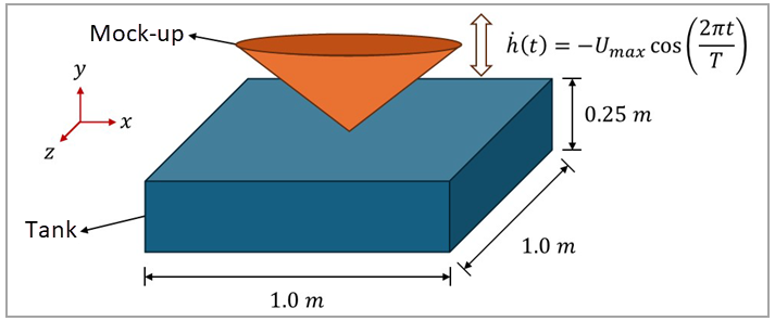
The experimental domain consists of a water tank and a mock-up with a small vertical gap from the water surface. The mock-up has a prescribed oscillatory translation with maximum entry-exit velocities of 0.6 m/s. The numerical adaptation of the problem in the LS-DYNA application was reduced to an axisymmetric problem with a quarter domain described by a rectangular prism with a conical cavity. The cavity represents the mock-up (conical body), and the lateral surfaces where the cavity is located are the symmetry surfaces. An initial level set is defined as 0.25 m to delimitate the air-water surface in the domain, and no gap is defined between this surface and the mock-up. Figure 257 illustrates the domain dimensions and boundary conditions.
Figure 257: Schematic of the test case, including domain geometry, main dimensions, and boundary conditions
The following table lists the material properties, geometric properties, and loading. The units for the current test case follow the International System of Units.
| Material Properties | Geometric Properties | Loading |
|---|---|---|
|
Fluid: Fluid density: (ρ) = 1000 kg/m3
Dynamic viscosity: (μ) = 0.001 Pa·s |
Geometry: Prism base dimensions: (Wp) = 0.50 m x 0.50 m
Prism height: (Hp) = 0.45 m
Mesh Size: Fluid boundary element size = 0.0025 m |
Conical Body: Oscillatory vertical velocity with amplitude of 0.6 m/s (Umax) and period of 0.5393 s (T)
Fluid: Gravity load (g) = 9.81 m/s2 Initial level set = 0.25 m |
Analysis Assumptions and Modeling Notes
The test case is based on a set of entry-exit experiments on a water tank that is equipped
with a motion generator, enforcing a purely vertical translation to the mock-ups (Breton et
al., 2020; Goron et al., 2023). The current case reproduces the experiment that used a
conical-shaped body with a maximum translational velocity of 0.6 m/s. The
prescribed vertical translation,  , of the lowest point of the mock-up is defined by the following
equation:
, of the lowest point of the mock-up is defined by the following
equation:
 | (88) |
Where  is the maximum vertical translation,
  is the maximum vertical velocity,
  is the period,
  is the time, and
  is a phase shifter. The vertical velocity,
  , can be obtained by deriving the translation function with respect to
time:
, can be obtained by deriving the translation function with respect to
time:
 | (89) |
Since the maximum velocity of the mock-up is 0.6 m/s and the maximum displacement is 0.0515 m, the period of the oscillatory motion profile can be calculated as 0.5393 s. The vertical hydrodynamic force acting on the mock-up is measured by piezoelectric load cells, used as a comparison for the numerical results.
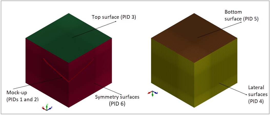
Six ICFD parts are defined to represent the conical body (IDs 1 and 2), the top surface (ID 3), the lateral surfaces (ID 4), the bottom surface (ID 5), and the symmetry surfaces (ID 6). An ICFD part volume (ID 77) is assigned within the six ICFD parts. These parts are meshed with 2D quadrilateral surface elements of size 0.0025 m. The bottom surface uses an ICFD material card (ID 2) that represents the free surface problem (FLG = 0). The other five parts use an ICFD material card with a density of 1000 kg/m3 and a dynamic viscosity of 0.001 Pa·s.
The boundary conditions are non-slip for the conical body (defined with *ICFD_BOUNDARY_NONSLIP) and free-slip for the remaining boundary surfaces (defined with *ICFD_BOUNDARY_FREESLIP). An oscillatory Y-velocity is prescribed to the conical body using *ICFD_CONTROL_IMPOSED_MOVE with a maximum velocity of 0.6 m/s and time period of 0.5393 s. The symmetry condition is added on the symmetry surfaces by constraining the translation of surface nodes in the X- and Z-direction using ICFD_BOUNDARY_PRESCRIBED_MOVEMESH. An initial level set surface is defined as the Y-plane using *ICFD_INITIAL_LEVELSET (normal in the Y-direction at the global origin). Gravity is included by prescribing a Y-acceleration of 9.81 m/s2 to all nodes using *LOAD_BODY_Y.
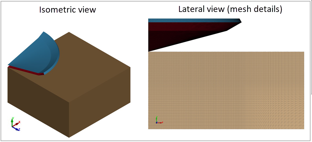
The keyword *MESH_VOLUME is defined within the six ICFD parts to select the region that must be meshed. Boundary-layer meshing refinements are performed by using *MESH_BL on the conical body and *MESH_BL_SYS on the symmetry surfaces. The keyword *ICFD_CONTROL_TIME is used to define the termination time of 0.2754 s and the time step of 0.00125 s. The solver keywords *ICFD_SOLVER_TOL_LSET, *ICFD_SOLVER_TOL_MOM, and *ICFD_SOLVER_TOL_PRE are used to set the convergence criteria to 1.0 · 10-12 and the maximum number of iterations allowed to 2000 for the advection equation for level set, the momentum equation and the Poisson equation for pressure.
Results Comparison
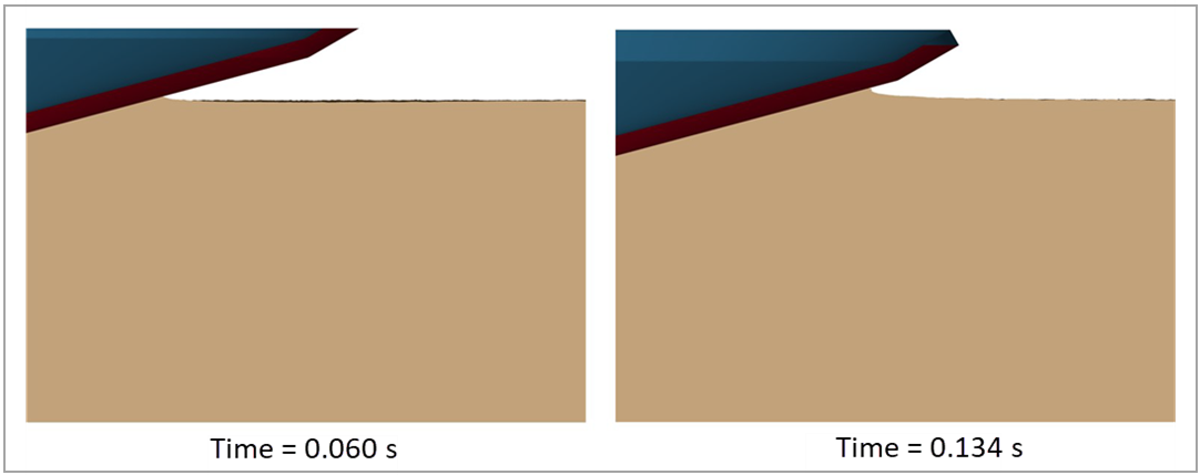
The fluid behavior for different mock-up positions is shown in Figure 260. Note that for the second moment, the mock-up has a velocity close to zero and starts the process of exiting the fluid.
The validation of the model is performed by comparing the vertical hydrodynamic force over time for the experiment and the LS-DYNA model solved with the ICFD solver. Since only a quarter domain is simulated, the force profile obtained from the LS-DYNA application must be multiplied by four. Figure 261 shows the vertical fluid force acting on the mock-up versus time for both cases, indicating a close agreement between the experiment and the LS-DYNA solution.
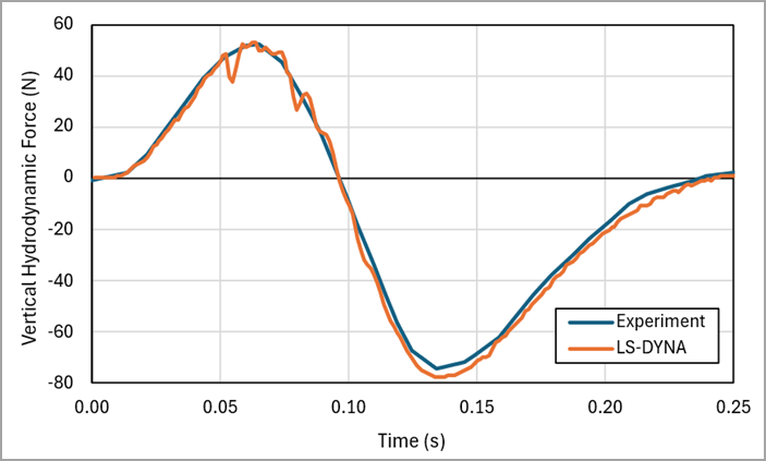
To quantify the error between the experimental and LS-DYNA results, the maximum and minimum vertical hydrodynamic force and their relative errors are calculated and shown in the following table. This comparison further verifies the excellent agreement between the force profiles.
| Results | Target | LS-DYNA | Error (%) |
|---|---|---|---|
| Name of result | Result value from experiment (N) |
Result value fromLS-DYNA application (N) | Percent error between Target and LS-DYNA application |
| Maximum vertical hydrodynamic force | 52.15 | 51.24 | -1.73% |
| Minimum vertical hydrodynamic force | -74.17 | -77.21 | 4.10% |