


VM-LSDYNA-FLUID-009
VM-LSDYNA-FLUID-009
Womersley Flow: Pulsative Flow in a Rigid Cylindrical Tube
Overview
| Reference: |
Truskey, D. A., Yuan, F., & Katz, D. F. (2004). Transport phenomena in biological systems. Pearson Prentice Hall. pp. 214–222. U.S. Food and Drug Administration. (2014, January). Reporting of computational modeling studies in medical device submissions: Draft guidance for industry and FDA staff. https://www.fda.gov/ Oberkampf, W. L., & Roy, C. J. (2010). Verification and validation in scientific computing. Cambridge University Press. |
| Analysis Type(s): | Incompressible CFD |
| Input Files: | Link to Input Files Download Page |
Test Case Description
This test case models the Womersley flow which consists of an oscillatory, fully developed laminar flow of a Newtonian fluid in a rigid cylindrical tube driven by a time-periodic pressure gradient. This problem is widely used as a benchmark in hemodynamics and CFD verification as it captures the effects of both viscous diffusion and pulsatile forcing which is relevant to arterial blood flow. The test objective is to validate the axial velocity profile in the tube for various phases.
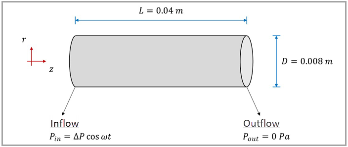
The tube, represented by a cylindrical domain, includes an inflow boundary with prescribed oscillatory pressure, an outflow boundary with prescribed pressure, and the remaining boundary with a non-slip condition. Figure 252 illustrates the domain dimensions and boundary conditions.
The following table lists the main parameters of the test case. The units for the current test case follow the International System of Units: length in m, time in s, mass in kg, force in N, and pressure in Pa.
| Geometric Properties | Material Properties | Loading |
|---|---|---|
|
Geometry: Tube radius ( Tube length ( Mesh size: Fluid boundaries element size = 0.0002 m |
Fluid: Fluid density ( Dynamic viscosity ( |
Fluid: Inflow oscillatory pressure ( Outflow pressure ( |


Analysis Assumptions and Modeling Notes
The governing flow behavior is characterized by two dimensionless quantities: the Reynolds number and the Womersley number. The Reynolds number is calculated to determine the flow regime:
 | (83) |
where
 is
the density of the fluid is
the density of the fluid |
 is
the characteristic diameter of the tube is
the characteristic diameter of the tube |
 is
the mean velocity of the flow is
the mean velocity of the flow |
and  is the dynamic viscosity of the fluid
 |
For a steady pipe flow, the laminar-turbulent transition occurs for a
Reynolds number of 2000. Since the Womersley solution assumes a laminar flow, a necessary
condition is  ≪ 2000. Since the periodic flow induces different
velocity fields through time, a safe laminar range for different Womersley numbers is
< 1000.
≪ 2000. Since the periodic flow induces different
velocity fields through time, a safe laminar range for different Womersley numbers is
< 1000.
While both the Womersley and Reynolds numbers quantify the relative
importance of unsteady inertial forces to viscous forces, the former is required when the
pressure drop exhibits periodicity, whereas only the Reynolds number is relevant when there is
no pulsatile pressure drop. The Womersley number  is calculated as:
 | (84) |
where
 is
the tube radius is
the tube radius |
 is
the oscillation frequency (calculated as 2π over the period) is
the oscillation frequency (calculated as 2π over the period) |
and  is the kinematic viscosity of the fluid (calculated as the ratio between dynamic viscosity,
, and
density, )
is the kinematic viscosity of the fluid (calculated as the ratio between dynamic viscosity,
, and
density, ) |
For small , the velocity profiles
are parabolic and nearly in phase with the pressure gradient (quasi-steady Poiseuille-like).
For moderate , the profiles are flatter, with central jetting and phase lag relative to pressure. For
large ,
plug-like velocity profiles dominate, and flow reversals may occur near the wall. The
Womersley number is 5.518 in the present case, which leads to velocity profiles that exhibit
phase lag and flow reversal during parts of the oscillation cycle.
Considering a laminar, linear, fully developed, unidirectional, axisymmetric flow through a rigid cylindrical tube, the Navier-Stokes equation can be simplified to:
 | (85) |
where
 and and  are the pressure and axial velocity profiles are the pressure and axial velocity profiles |
 and and  are the axial and radial coordinates are the axial and radial coordinates |
and  is the time is the time |
The pressure gradient portion can be represented by:
 | (86) |
where
 is the imaginary number is the imaginary number |
 is the pressure drop amplitude through the tube is the pressure drop amplitude through the tube |
and  denotates the real part denotates the real part |
The analytical velocity field  in cylindrical coordinates is then obtained by solving the unsteady
Navier–Stokes equation:
in cylindrical coordinates is then obtained by solving the unsteady
Navier–Stokes equation:
 | (87) |
where  is the Bessel function of the first kind of order zero.
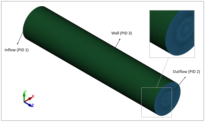
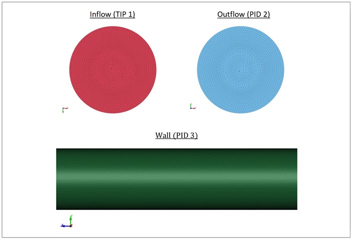
Three ICFD parts are defined to represent the tube inlet (ID 1), outlet (ID 2), and wall (ID 3). These parts are meshed with 2D triangular surface elements with size of 0.0002 m. An ICFD part volume (ID 10) is assigned within the three ICFD parts. These parts use the ICFD material card with a flow density of 1060 kg/m3 and a dynamic viscosity of 0.0035 Pa⋅s.
The inlet boundary condition is the oscillatory pressure profile with an amplitude of 3 Pa and a frequency of 2π rad/s defined by *ICFD_BOUNDARY_PRESCRIBED_PRE. The outlet boundary condition is the pressure of zero defined by *ICFD_BOUNDARY_PRESCRIBED_PRE. The boundary condition for the tube wall was defined as non-slip with *ICFD_BOUNDARY_NONSLIP.
The keyword *MESH_VOLUME is defined within the three ICFD parts to select the region that must be meshed. Boundary-layer meshing refinements are performed by using *MESH_BL on the wall and *MESH_BL_SYS on the inlet and outlet. The keyword *ICFD_CONTROL_TIME is used to define the termination time of 4.0 s and the time step of 0.001 s. The solver keywords *ICFD_SOLVER_TOL_MOM and *ICFD_SOLVER_TOL_PRE are used to manually input the convergence criteria to 1.0 ⋅ 10-11 for the momentum equation and the Poisson equation for pressure.
Results Comparison
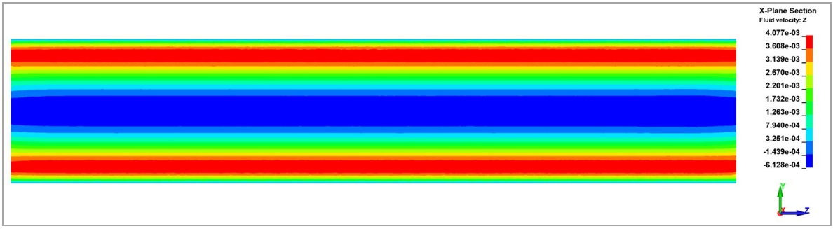
The contour plot for the axial velocity during phase 0 (t = 3 s) is shown in Figure 255. The velocity profile is axisymmetric due to the geometry, boundary conditions, and laminar flow. For this specific phase, the velocity is positive close to the wall and slightly negative (reverse flow) in the central axis.
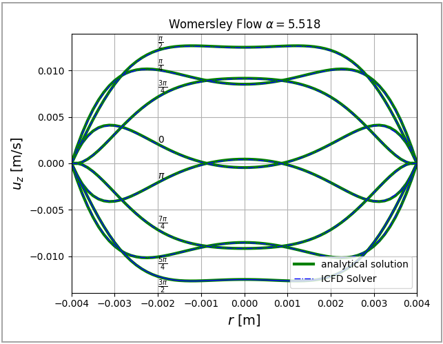
The validation of the model is performed by comparing the axial velocity profile at the mid-length of the tube (z = 0.02 m) for the analytical solution and for the LS-DYNA model. A Python script comparing the analytical and LS-DYNA velocity profiles for different phases is attached with the input files. Eight timesteps are selected to reproduce the flow behavior during distinct phases: 3.0 s (phase 0), 3.125 s (phase π/4), 3.25 s (phase π/2), 3.375 s (phase 3π/4), 3.5 s (phase π), 3.625 s (phase 5π/4), 3.75 s (phase 3π/2), 3.875 s (phase 7π/4). Figure 256 shows the axial velocity versus radial coordinate for analytical and LS-DYNA solutions, indicating a close agreement for all phases.
Figure 256: Axial velocity versus radial coordinate at the mid-length of the tube (z = 0.02 m) for different flow phases
To quantify the error between the analytical and LS-DYNA solutions, the root mean square error (RMSE), maximum error, and minimum error for the eight axial velocity profiles are calculated and showed in the following table. This comparison further verifies the excellent agreement between the velocity profiles.
In the table below, the root mean square error (RMSE), maximum error, and minimum error between the axial velocity profiles calculated by the analytical solution and by the ICFD solver in LS-DYNA for different flow phases
| Flow Phase | RMSE between Velocity Profiles (m/s) | Maximum Error between Velocity Profiles (m/s) | Minimum Error between Velocity Profiles (m/s) |
|---|---|---|---|
| Phase 0 | 5.09 ⋅ 10-5 | 1.26 ⋅ 10-4 | 2.76 ⋅ 10-5 |
| Phase π/4 | 5.75 ⋅ 10-5 | 1.20 ⋅ 10-4 | 2.92 ⋅ 10-5 |
| Phase π/2 | 5.08 ⋅ 10-5 | 7.51 ⋅ 10-5 | 5.15 ⋅ 10-6 |
| Phase 3π/4 | 4.33 ⋅ 10-5 | 6.04 ⋅ 10-5 | 1.36 ⋅ 10-6 |
| Phase π | 4.35 ⋅ 10-5 | 1.14 ⋅ 10-4 | 4.09 ⋅ 10-7 |
| Phase 5π/4 | 3.78 ⋅ 10-5 | 1.09⋅ 10-4 | 2.17 ⋅ 10-6 |
| Phase 3π/2 | 1.98 ⋅ 10-5 | 4.65 ⋅ 10-5 | 2.40 ⋅ 10-7 |
| Phase 7π/4 | 1.72 ⋅ 10-5 | 6.09 ⋅ 10-5 | 6.28 ⋅ 10-7 |