


VM-LSDYNA-SPH-001
VM-LSDYNA-SPH-001
2D Laminar Couette Flow Simulation (SPH)
Overview
| Reference: |
Munson, B. R., Okiishi, T. H., Huebsch, W. W., & Rothmayer, A. P. (2013). Fundamentals of fluid mechanics (7th ed.). Wiley & Sons. https://bcs.wiley.com/he-bcs/Books?action=index&itemId=1118318676&bcsId=7938 Monaghan, J. J. (1994). Simulating free surface flows with SPH. Journal of Computational Physics, 110(2), 399–406. |
| Analysis Type(s): | Laminar Couette Flow Simulation using SPH |
| Input Files: | Link to Input Files Download Page |
Test Case
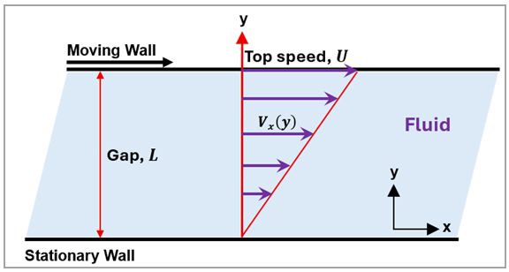
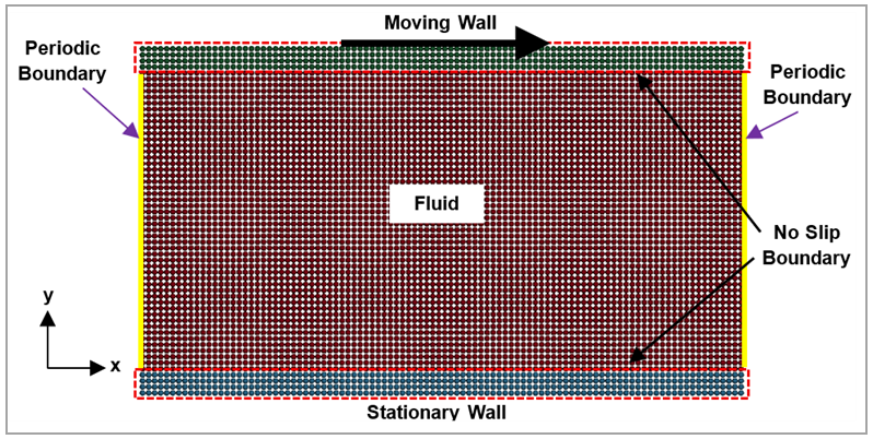
The simulation models classical Couette flow, representing a viscous, incompressible fluid confined between two parallel plates. The bottom plate is stationary, while the top plate moves at a constant horizontal velocity, generating a linear shear-driven flow in the fluid layer. The domain geometry is two-dimensional (2D), and flow is driven solely by the relative motion of the plates without any applied pressure gradient or gravity. A no-slip condition is applied at both plates, ensuring that the fluid velocity roughly matches that of the adjacent surfaces. Periodic boundary conditions are applied on the left and right sides to eliminate end effects and simulate an infinite span in the flow direction. See the schematic and the properties table below.
Figure 262: Schematic of classical Couette laminar flow between parallel plates with no gravity or pressure gradient in vertical direction
| Material Properties | Geometric Properties | Loading |
|---|---|---|
|
Density: 0.001 kg/cm3 or 1000 kg/m3 in SI, representing water Pressure cutoff: -500 kg/(cm.s2) or -50 k Pa in SI Viscosity coefficient: 10E-5 kg/(cm.s) or 0.001 Pa.s in SI Initial bulk modulus (at zero pressure): 1500 kg/(cm.s2) or 150 kPa in SI Pressure derivative of the bulk modulus (at zero pressure): 7 (dimensionless) |
Height of the domain (gap between plates): 1 cm Length of the domain (along the flow direction): 2 cm Uniform SPH particle spacing: 0.02 cm Fluid particle count: 5000 (resolution of 50 × 100) Wall particle count: 400 (resolution of 4 × 100) |
No pressure gradient No gravity Moving top wall with no slip condition Velocity of the moving wall (top) in X direction = 0.5 cm/s
Boundary Conditions Periodic boundary condition applied on left (inlet) and right (outlet) Stationary bottom wall with no slip condition |
Analysis Assumptions and Modeling Notes
Starting from the simplified form of the Navier–Stokes equations for steady, incompressible, fully developed Couette flow
 | (90) |
where  is the fluid velocity in positive x direction as shown in Figure 263. Integrating Equation 90 twice with respect to y:
 | (91) |
Implemented boundary conditions are
 | (92) |
When boundary conditions are applied, the analytical solution becomes
 | (93) |
In this case study where  and
and  ,
,
 | (94) |
In various engineering applications, the Reynolds number is crucial for understanding
fluid behavior. This test case uses a low Reynolds number of 100.  was calculated using the equation
 | (95) |
where 𝛒 is the fluid density,  is the speed of the top moving plate,
  is the gap size—the characteristic length in this case study—and
𝛍 represents the dynamic viscosity of the fluid.
is the gap size—the characteristic length in this case study—and
𝛍 represents the dynamic viscosity of the fluid.
True incompressibility is computationally prohibitive. In SPH simulations, incompressible
flow is approximated by using an artificial bulk modulus  that ensures the fluid’s Mach number
  remains much less than 0.01 (to 0.1). This is achieved by selecting
such that the artificial speed of sound
remains much less than 0.01 (to 0.1). This is achieved by selecting
such that the artificial speed of sound  is significantly greater than the maximum flow velocity . In this model,
  and
and  , giving an artificial sound speed of
  . Given the velocity of the top plate
  , the resulting Mach number is
  , which is well within the acceptable range for weakly compressible SPH. This
approach keeps density fluctuations minimal (typically below 1%) and is widely accepted in the
SPH community (Monaghan, 1994 for example) as a computationally efficient alternative to
modeling strictly incompressible fluid. That is, the weakly compressible SPH (WCSPH) approach
used by Monaghan approximates incompressibility by keeping density variations small, typically
below 1% or 2%, ensuring density remains tightly clustered around the reference value.
, which is well within the acceptable range for weakly compressible SPH. This
approach keeps density fluctuations minimal (typically below 1%) and is widely accepted in the
SPH community (Monaghan, 1994 for example) as a computationally efficient alternative to
modeling strictly incompressible fluid. That is, the weakly compressible SPH (WCSPH) approach
used by Monaghan approximates incompressibility by keeping density variations small, typically
below 1% or 2%, ensuring density remains tightly clustered around the reference value.
For the simulation, *BOUNDARY_SPH_NOSLIP is used. This test case assumes both fluid density (incompressible flow) and fluid viscosity are constant. Shear stress is linearly proportional to strain rate (Newtonian fluid). The flow is smooth and orderly with no turbulence (laminar flow). Fluid velocity at the boundary equals the wall velocity (no-slip condition at the walls). There is no gravity or pressure gradient in the vertical (y) direction. Therefore, the flow is driven solely by the motion of the top plate. Properties do not change with time (steady-state or fully developed flow), and thermal effects and compressibility are neglected.
Regarding modeling, the entire domain is discretized using uniformly spaced SPH nodes. A 2D simulation is achieved by using only one SPH node in the z direction. The top and bottom plates are parallel, separated by a fixed gap. The model uses the [kg–cm–s] unit system. However, other unit systems (SI for example) can be used, provided the Reynolds number is maintained at a low value (for example, Re = 100, as used in this case study).
Results Comparison
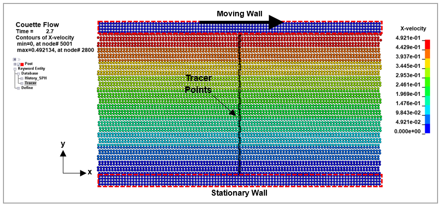
To verify the accuracy of the SPH-based Couette flow simulation, velocities were extracted along the vertical centerline of the domain at two time instances, 1.8 s and 2.7 s (Figure 264), using tracer points as shown in Figure 265.
Figure 264: Predicted velocities (cm/s) at different tracer points as a function of time compared with the analytical solution at 1.8 s and 2.7 s.
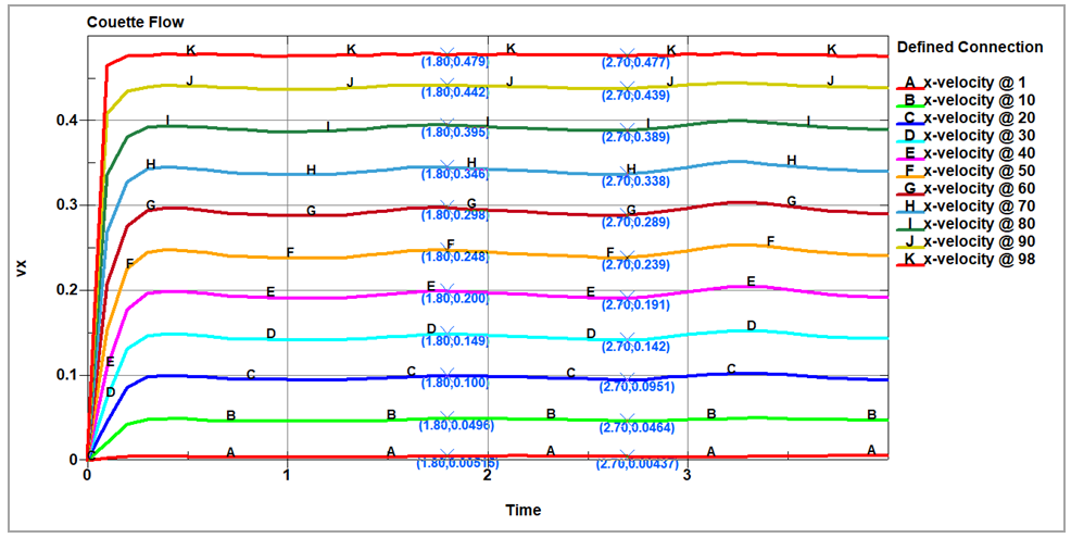
Figure 265: Tracer points used to extract predicted flow velocities along the vertical centerline of the domain
A linear fit was then applied to each profile to compare with the analytical solution as shown in Figure 266.
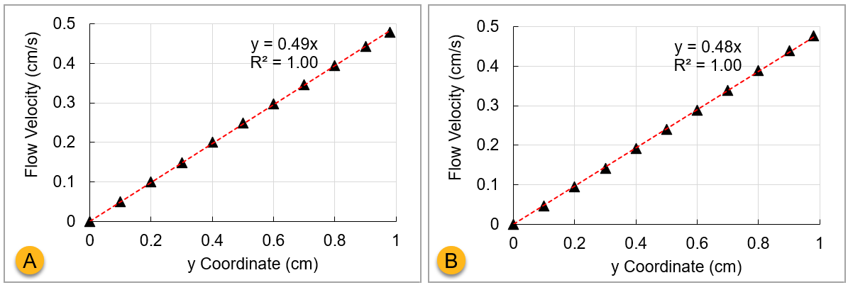
The results show that the velocity profiles at both times exhibit linear behavior with respect to the y coordinate consistent with the theoretical expectations for steady Couette flow. As summarized in the results table below, the extracted slopes were 0.49 at 1.8 s and 0.48 at 2.7 s. These values closely match the analytical slope of 0.5, confirming that the SPH formulation accurately captures the shear-driven flow.
| Results | Target | LS-DYNA | Error (%) |
|---|---|---|---|
| Slope of the velocity profile at vertical centerline at time 1.8 s | 0.5 | 0.49 | 2% |
| Slope of the velocity profile at vertical centerline at time 2.7 s | 0.5 | 0.48 | 4% |