


VM-LSDYNA-FLUID-008
VM-LSDYNA-FLUID-008
2D Passive Scalar Transport in a Laminar Channel Flow
Overview
| Reference: | Bird, R.B., Stewart, W.E., & Lightfoot, E.N. (2002). Transport phenomena (2nd edition). John Wiley & Sons, Inc. |
| Analysis Type(s): | Incompressible CFD |
| Input Files: | Link to Input Files Download Page |
Test Case
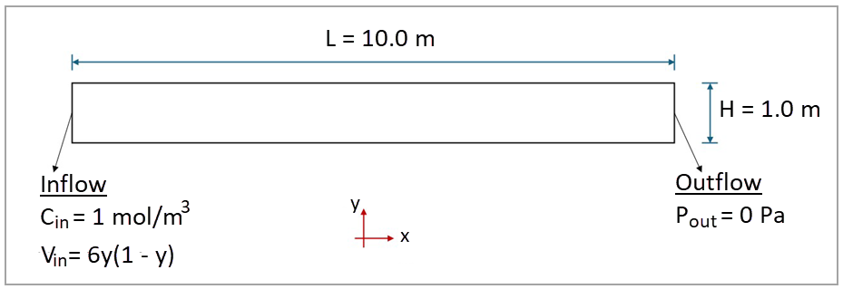
This test case models the transport of a passive scalar (species) in a two-dimensional, incompressible, steady, laminar flow inside a channel. The objective is to validate the final species concentrations at mid-length of the channel. The channel, represented by a rectangular domain, includes an inflow boundary (left edge) with prescribed species concentration and velocity, an outflow boundary (right edge) with prescribed pressure, and the two remaining boundaries (top and bottom edges) with non-slip conditions. The initial species concentration is zero in the whole domain.
The table below lists the main parameters of the test case, and Figure 247 illustrates the domain dimensions and boundary conditions. The units for the current test case follow the International System of Units (length in m, time in s, mass in kg, force in N, and pressure in Pa).
| Material Properties | Geometric Properties | Loading |
|---|---|---|
|
Fluid: Fluid density = 1.0 kg/m3 Dynamic viscosity = 0.02 Pa⋅s Scalar: Mass diffusion = 0.01 m/s2 |
Geometry: Channel height = 1.0 m Channel length = 10.0 m Mesh size: Fluid boundaries element length = 0.025 m |
Fluid: Inflow concentration = 1.0 mol/m3 Inflow average velocity = 1.0 m/s Outflow pressure = 0 Pa |
Figure 247: Schematic of the test case, including domain geometry, main dimensions, and boundary conditions
Analysis Assumptions and Modeling Notes
The Reynolds number is calculated to determine the flow regime
 | (76) |
where  is the density of the fluid,
  is the characteristic length of the channel,
  is the inlet flow mean velocity, and
  is the dynamic viscosity of the fluid. For a laminar flow, the Reynolds
number should be lower than 2100. The Reynolds number is 500 for the current test case, which
indicates that the channel flow is laminar.
is the dynamic viscosity of the fluid. For a laminar flow, the Reynolds
number should be lower than 2100. The Reynolds number is 500 for the current test case, which
indicates that the channel flow is laminar.
When considering a steady laminar flow, the fluid velocity profile through the channel,
 , can be described as the fully developed Poiseuille flow
 | (77) |
The 2D transient convection-diffusion equation for a passive scalar in a laminar channel flow is given by
 | (78) |
Where  is the scalar concentration, and
  is the mass diffusivity of the scalar. To solve this equation, the boundary
and initial conditions of the passive scalar should be evoked. The scalar concentration is
is the mass diffusivity of the scalar. To solve this equation, the boundary
and initial conditions of the passive scalar should be evoked. The scalar concentration is
 (1.0 mol/m3) at the inlet, the transverse
diffusive flux is zero at the walls, and the axial diffuse flux is zero at the outlet
(1.0 mol/m3) at the inlet, the transverse
diffusive flux is zero at the walls, and the axial diffuse flux is zero at the outlet
 | (79) |
 | (80) |
 | (81) |
The initial concentration of scalar is zero in the entire domain is
 | (82) |
Considering the convection-diffusion equation, the Poiseuille flow velocity profile, the boundary conditions, and the initial scalar concentration, the semi-analytical solution can be obtained using a numerical method. The Finite Differences Method (FDM) was used to find the concentration profiles at several x locations, which were used to validate the LS-DYNA model. A Python script covering all steps of the FDM solution is attached with the input files.
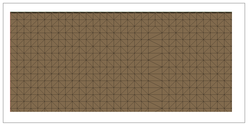
Three ICFD parts are defined to represent the channel inlet (ID 1), outlet (ID 2), and walls (ID 3). These parts are meshed with 1D surface elements with a length of 0.025 m. An ICFD part volume (ID 10) is assigned within the three ICFD parts. These parts use the ICFD material card with a flow density of 1 kg/m3 and a dynamic viscosity of 0.02Pa⋅s. The keyword *ICFD_MODEL_SPECIES_TRANSPORT is used to reproduce the behavior of one passive species with a mass diffusion of 0.01 m/s2, being referenced by the ICFD material model. The species concentration is initialized with *ICFD_INITIAL_SPTRANSP within the part volume.
The inlet boundary conditions are the Poiseuille flow velocity profile defined by *ICFD_BOUNDARY_PRESCRIBED_VEL and the species concentration of 1.0 mol/m3 defined by *ICFD_BOUNDARY_PRESCRIBED_SPTRANSP_CONC. The outlet boundary condition is the pressure of zero defined by *ICFD_BOUNDARY_PRESCRIBED_PRE. The boundary condition for the channel walls was defined as non-slip with *ICFD_BOUNDARY_NONSLIP.
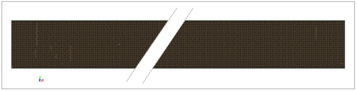
The keyword *MESH_VOLUME is defined within the three ICFD parts to select the region that must be meshed. Boundary-layer meshing refinements were performed by using *MESH_BL on the walls and *MESH_BL_SYS on the inlet and outlet. The keyword *ICFD_CONTROL_TIME was used to define the termination time of 5.01 s and the time step of 0.001 s.
Results Comparison
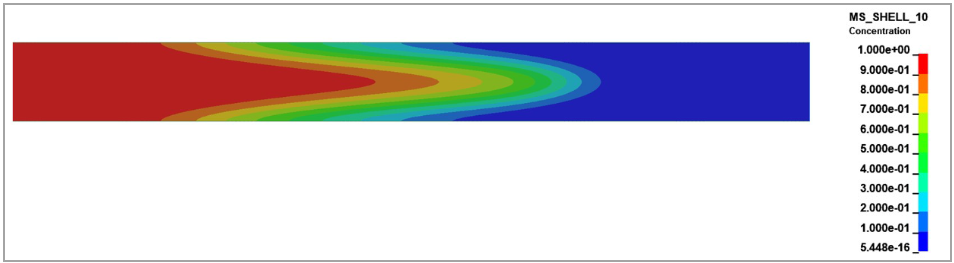
The contour plot for the species concentration is shown in Figure 250. The concentration profile is symmetric around y = 0.5 m due to the geometry, boundary conditions, and laminar flow. At t = 5 s, the domain is characterized by an initial region where the concentration is equal to the inlet concentration (1 mol/m3), a middle region where the concentration is still transient (between 0 and 1 mol/m3), and an end region where the concentration is equal to the outlet concentration (0 mol/m3).
The validation of the model is performed by comparing the final species concentration profile at the mid-length of the channel (x = 5 m) for the semi-analytical solution solved using FDM and for the LS-DYNA model solved with the ICFD solver. Figure 251 shows the species concentration versus y coordinate for both cases, indicating a close agreement between the semi-analytical and LS-DYNA solutions.
Figure 251: Final species concentration versus y coordinate at the mid-length of the channel (x = 5 m)
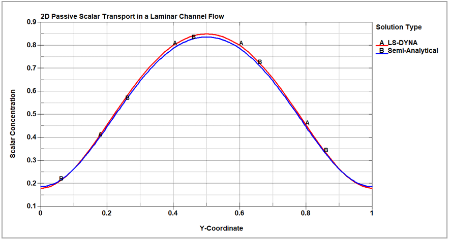
To quantify the error between the semi-analytical and LS-DYNA solutions, the concentration values for five data points are compared and their relative errors are calculated in the results table below. The maximum error of 3.95% is located on the channel wall, while most points have errors lower than 2%.
| Results | Target (mol/m3) | LS-DYNA (mol/m3) | Error (%) |
|---|---|---|---|
|
Final concentration (x = 5 m, y = 0 m) | 0.188 | 0.180 | 3.95% |
|
Final concentration (x = 5 m, y = 0.25 m) | 0.550 | 0.561 | 1.98% |
|
Final concentration (x = 5 m, y = 0.5 m) | 0.837 | 0.851 | 1.66% |
|
Final concentration (x = 5 m, y = 0.75 m) | 0.550 | 0.561 | 1.98% |
|
Final concentration (x = 5 m, y = 1 m) | 0.188 | 0.180 | 3.89% |
The general agreement between concentration profiles can be further verified when the mean relative error is calculated using all mid-length data points. When the final species concentration at the mid-length of the channel (x = 5 m) is compared for all data points, the mean relative error is 1.61%.