This section introduces the harmonic cyclic symmetry analysis capability with an example problem. The example presents a simplified ring-strut-ring structure used in many rotating-machinery applications.
The component is a simplified fan inlet case for a military aircraft engine. As part of the design process for the assembly, the harmonic response characteristics of the inlet case may be investigated, as shown in this example.
The geometric and material properties used for the harmonic cyclic analysis are the same as used in Example Modal Cyclic Symmetry Analysis.
All applicable degrees of freedom are used for the cyclic symmetry edge-component pairs. The harmonic response to a pressure load applied on the assembly is computed.
Use the input file given below (input_cyclicExample03.dat, download: input_cyclicExample03.zip) to perform the example harmonic cyclic symmetry analysis. The file contains the complete geometry, material properties, and solution options for the finite element model.
! Harmonic cyclic symmetry analysis example using a ring-strut-ring configuration.

! Set plot options.
/view,1,1,1,2
/plopts,minm,0
/plopts,date,0
/plopts,title,0
/plopts,logo,0
/pnum,real,1
/number,1

! Generating geometry and boundary conditions.
genGeometry = 1

*if, genGeometry, eq, 1, then

    ! Define geometry parameters.
    r1 = 5         ! Inner radius.
    r2 = 10        ! Outer radius.
    d1 = 2         ! Thickness.
    nsect = 24     ! Number of sectors.
    alpha_deg = 360 / nsect     ! Sector angle in degrees.
    alpha_rad = 2*acos(-1) / nsect     ! Sector angle in radians.

    ! Use cylindrical coordinate system.
    /prep7
    csys,1

    ! Create keypoints and define geometry.
    k,1,0,0,0
    k,2,0,0,d1
    k,3,r1,0,0
    k,4,r1,0,d1
    l,3,4
    arotat,1,,,,,,1,2,alpha_deg/2
    k,7,r2,0,0
    k,8,r2,0,d1
    l,7,8
    arotat,5,,,,,,1,2,alpha_deg/2
    arotat,2,,,,,,1,2,alpha_deg/2
    arotat,6,,,,,,1,2,alpha_deg/2
    a,5,6,10,9

    ! Set mesh options and define element types.
    mshkey,1
    et,1,181         ! Element type: shell-181.
    r,1,0.20         ! Thickness of the inner and outer rings.
    r,2,0.1          ! Thickness of the strut.
    esize,0.5        ! Element size.

    ! Define material properties and apply thermal loads.
    mp,ex,1,10e6     ! Young's modulus.
    mp,prxy,1,0.3    ! Poisson's ratio.
    mp,dens,1,1e-4   ! Density of the material.

    ! Apply thickness to inner and outer rings.
    asel,,,,1,4
    aatt,,1

    ! Apply thickness to strut.
    asel,,,,5
    aatt,,2
    allsel

    ! Mesh the areas.
    amesh,all

    ! Apply Dirichlet boundary conditions.
    ! Constrain all degrees of freedom at a keypoint on the inner ring.
    dk,5,all,0

    ! Save the model database.
    cdwrite, comb, cyclicExample03, cdb

*else
    cdread, comb, cyclicExample03, cdb,,,
*endif

! Configure cyclic symmetry analysis.
cyclic
/cycexpand,,on     ! Enable full model visualization.
eplot
cyclic,status      ! Display cyclic symmetry status.
cycopt,status      ! Display cyclic symmetry options.
finish

! Solve the harmonic cyclic symmetry analysis.
/solution

! Specify harmonic analysis option and frequency sweep values.
antype,harmic
hropt,full
harfrq,860,878
nsub,9             ! Number of subdivisions between the frequencies.

! Apply pressure load on the outer surface area.
asel,s,area,,2
asel,a,area,,4

! Apply pressure loading to sector number 3.
cycopt,ldsect,3
sfa,all,,pres,-124
asel,all

solve
finish

! Post-process the results.
/post1
! Read results for substep 3 - excitation frequency of 866 Hz.
set,,3
plns,u,sum,1
*get, maxvalusum, plnsol,0,max
finish

! Go to time/frequency history postprocessor.
/post26
/com, Postprocessing
! Extract X and Y displacement of node #34 on sector #3.
nsol,2,34,u,x,ux_34,3
nsol,3,34,u,y,uy_34,3

! Plot the ux and uy displacements of node #34.
plvar,2,3

*get, maxvalux34, VARI, 2, extrem, vmax
*stat, maxvalux34
*get, maxvaluy34, VARI, 3, extrem, vmax
*stat, maxvaluy34

finish
The following table describes the input listing and the steps involved in the example harmonic cyclic symmetry analysis in detail.
| Step | Step Description | Description |
| 1. | Generate the model. | ET, MP, AMESH |
| 2. | Specify a cyclic symmetry analysis and configure the database accordingly. | CYCLIC |
| 3. | Activate cyclic symmetry graphical expansion. | /CYCEXPAND,,ON |
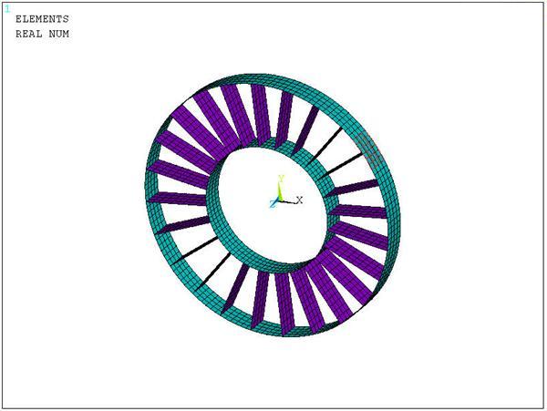
| 4. | Plot the elements. Figure 5.5: Element Plot Showing Pressure Load on Sector 3 shows an element plot showing pressure load on sector 3. | EPLOT |
| 5. | List the cyclic status. | CYCLIC,STATUS |
| 6. | List the cyclic solution option settings. | CYCOPT,STATUS |
| 7. | Solve the harmonic cyclic symmetry analysis with non-cyclic loading. |
CYCOPT,LDSECT |
| 8. | Enter database results postprocessor. | /POST1 |
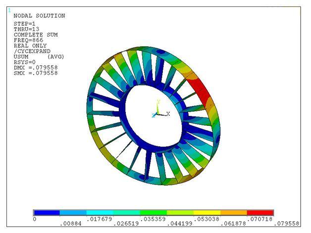
| 9. | Read results for sub step 3 – Frequency = 866. | SET,1,3 |
| 10. | Plot the displacement sum contour. Figure 5.6: Contour Plot of Displacement Sum at Frequency of 866 HZ shows a contour plot of displacement sum at frequency = 866 HZ. | PLNSOL,U,SUM |
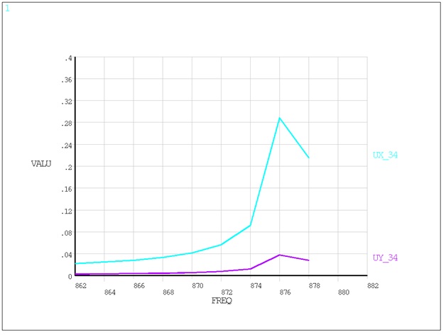
| 11. | Enter time/frequency history postprocessor. | /POST26 |
| 12. | Store nodal data from results file for node 34, sector 3. | NSOL,2,34,u,x,UX_34,3 |
| NSOL,3,34,u,y,UY_34,3 | ||
| 13. | Plot frequency versus displacement. Plot at node 34. Figure 5.7: Displacement Plot as a Function of Excitation Frequency shows the displacement plot as a function of the excitation frequency. | PLVAR,2,3 |
The results of your analysis should match those shown below: