


If your FreeFlow project was opened through Workbench, an External Coupling component automatically appears in the FreeFlow Data panel. For FreeFlow projects coupled with Ansys Mechanical through Workbench, this component enables you to define the kind of data gets shared between the programs, such as the geometry loads.
For FreeFlow projects that are coupled with other Ansys products (not including Mechanical) through Workbench, this component can be ignored.
What would you like to do?
Ansys Workbench is a product you can use to more easily connect, share, automate, and keep organized data across various programs. When used with FreeFlow, Workbench can help you accomplish many time-saving tasks like the ones described in the sections below.
Tip: To learn which versions of Ansys -including Workbench, Discovery, Mechanical, Fluent, and other products- are compatible with this version of FreeFlow, refer to System Requirements.
This section covers the following topics:
FreeFlow INTEGRATION IN WORKBENCH
WORKBENCH INTEGRATION IN FreeFlow
MAXIMIZE THE DESIGN OF YOUR GEOMETRY COMPONENTS BY USING ANSYS DISCOVERY
PARAMETERIZE SIMULATION AND SETUP COMPONENTS BY USING ANSYS DESIGNXPLORER
ABOUT DEFINING EXTERNAL COUPLING OPTIONS
DEFINE OPTIONS FOR EXTERNAL COUPLING
ABOUT THE HEAT TRANSFER COEFFICIENT (HTC) COMPONENT
FreeFlow INTEGRATION IN WORKBENCH
Once you open Workbench and create a new Project, you can from the Toolbox panel, expand the Analysis Systems item, and then drag and drop Fluids (FreeFlow) to the Project Schematic (Figure 3.116: Fluids (FreeFlow) as an Ansys Workbench Component).
Note: This item will be referred to as the "FreeFlow" block for simplicity.
This creates a link between your Workbench project and the FreeFlow program. From here, you can either start a new FreeFlow project from within Workbench (Edit), or import a FreeFlow project into Workbench that you have already set up (Import Setup).
The link between your Workbench project and your FreeFlow project means that data will be automatically transferred between the two programs. In addition, it exposes FreeFlow input and output parameters, so you can explore Workbench capabilities such as evaluating multiple design points, creating FreeFlow cases automatically, and then running them through the weekend.
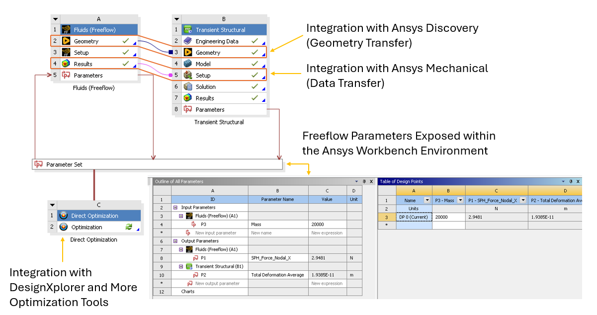
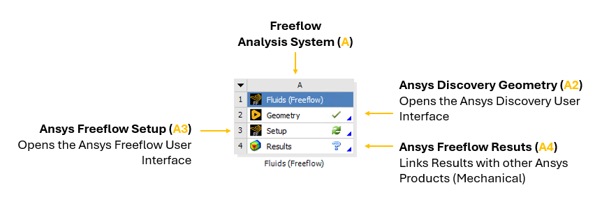
The FreeFlow Analysis System block (A) is made up of the components described in Figure 3.117: FreeFlow Analysis System Block in Workbench.
By interacting with the FreeFlow Analysis System block, and linking other items from the Workbench Analysis System-such as the Transient Structural block or the Static Structural block-to the FreeFlow items listed, you can have Workbench perform many different tasks in FreeFlow. This includes one-way coupled approaches with Ansys Mechanical, standalone parametric studies, and more.
Note: In FreeFlow, projects coupled with Ansys Workbench use Ansys Discovery as default for Geometry imports and conversions. Therefore, if Ansys Discovery is not installed, you will get an error message when trying to convert geometries into .STL in FreeFlow-Workbench coupled projects.
WORKBENCH INTEGRATION IN FreeFlow
If you have linked to FreeFlow from within Workbench, an External Coupling entry will appear in the FreeFlow Data panel (Figure 3.118: FreeFlow connected to Mechanical via Workbench, showing a new External Coupling entry).
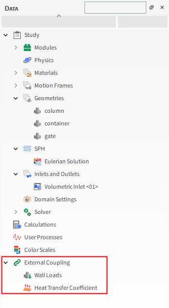
For FreeFlow projects opened through Workbench that are not coupled with Ansys Mechanical, this component will still appear in the Data panel but can be ignored.
See Also:
MAXIMIZE THE DESIGN OF YOUR GEOMETRY COMPONENTS BY USING ANSYS DISCOVERY
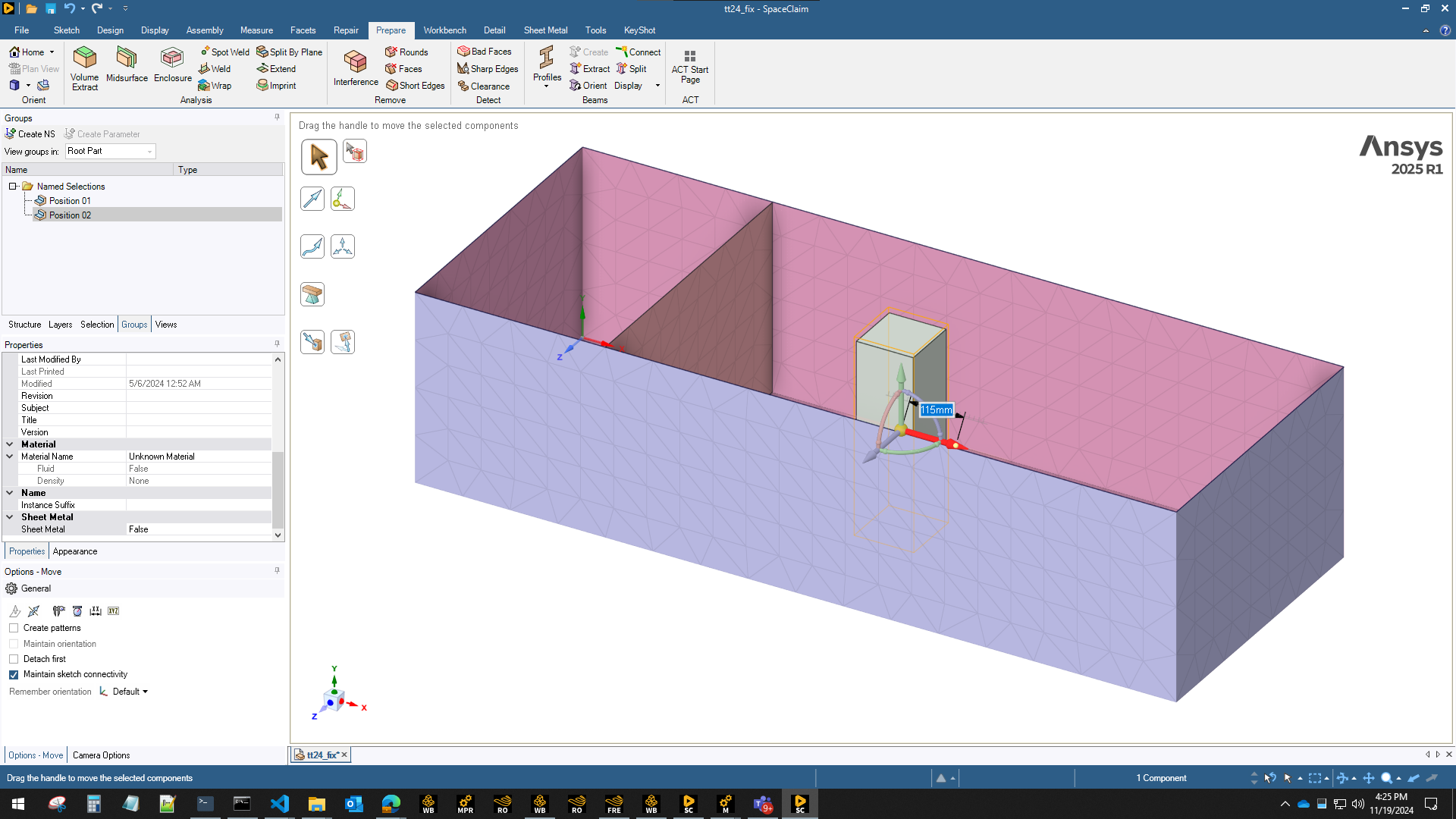
This is accomplished through Workbench by connecting your FreeFlow project with Ansys Discovery 3D geometry files, thereby enabling you to change equipment components in Ansys Discovery (Figure 3.119: Geometry component being modified in Discovery) and have those geometry changes be automatically updated in your FreeFlow project.
Note: In Ansys FreeFlow, projects coupled with Ansys Workbench use Ansys Discovery as default for Geometry imports and conversions. Therefore, if Ansys Discovery is not installed, you will get an error message when trying to convert geometries into .STL in FreeFlow-Workbench coupled projects.
PARAMETERIZE SIMULATION AND SETUP COMPONENTS BY USING ANSYS DESIGNXPLORER
This is accomplished through Workbench by connecting your FreeFlow project with Ansys DesignXplorer, which enables you to set design goals and get immediate feedback on proposed changes. DesignXplorer includes correlation, design of experiments, response surface creation and analysis, optimization and six sigma analysis. In addition, integration with other Ansys products like Discovery ensures that any geometry changes made are automatically updated in your FreeFlow project.
Using DesignXplorer through Workbench can be especially helpful when testing how small changes in geometry angles, sizes, or placements affects your simulation.
CONDUCT FEA ANALYSIS OF FLUID ACTING UPON GEOMETRY COMPONENTS BY USING ANSYS MECHANICAL
By using Workbench to connect your FreeFlow project with Ansys Mechanical, you can have Mechanical predict the stress and strain response of your geometry components when they are subjected to the loads that are calculated in FreeFlow.
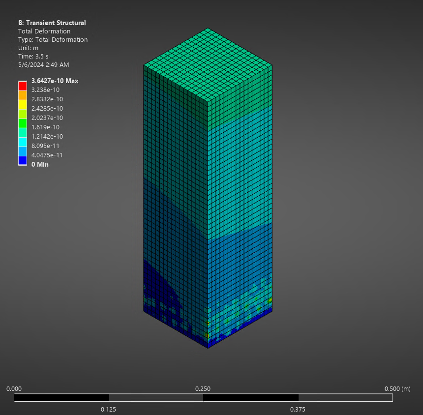
Workbench does this by first having FreeFlow calculate the SPH elements forces and pressures on the geometry component. Next, it automatically exports that data from FreeFlow to Mechanical through Workbench, where Mechanical then uses those forces and pressures to perform static or transient (over a time range - Figure 3.120: Example of a transient structural FEA analysis) structural analysis on the component. This approach is useful for analyzing the stress effects of fluids over structures, for example.
ABOUT DEFINING EXTERNAL COUPLING OPTIONS
If you have an External Coupling component in your FreeFlow Data panel, this indicates that your FreeFlow project has been opened through Workbench. Although it will appear for any type of coupled project that you open through Workbench, it is designed to work only with FreeFlow projects that are coupled specifically with Ansys Mechanical.
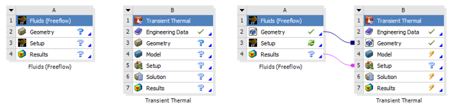
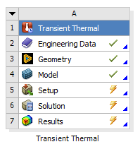
Tip: As a best practice, it is important to open workbench, insert the FreeFlow and Mechanical components (left figure below showing unattached FreeFlow and Transient Thermal), then manually open an save FreeFlow's project, and only then manually link FreeFlow to Mechanical (right figure below showing FreeFlow and Transient Thermal attached).
For projects coupled with Mechanical, defining the options for this component enables you to determine what kind of SPH data to share, as described below.
For all other coupled projects, including those with only Ansys Discovery, this External Coupling component can be ignored.
ABOUT THE GEOMETRY LOADS COMPONENT
When you define options for the Geometry Loads component, you choose the geometry component(s) for which you want to share fluid load data with the coupled Ansys Mechanical program, and the simulation time frame during which you want data (Figure 3.122: External Coupling entity expanded to show the Geometry Loads component).
By limiting the data you share to only what you require for your analyses, you reduce the amount of time the coupled simulation will take to process.
GEOMETRY LOAD PARAMETERS
Use the image above and table below to help you understand how to define options for Geometry Loads.
Table 1: Geometry Loads Parameter Definitions
|
Setting |
Description |
Range |
|---|---|---|
|
Select Geometries |
Enables you to choose which geometry data will be shared during the coupled simulation. |
Turns on or off |
|
Domain Range |
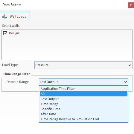
Defines what time steps of the simulation are included in the data to be shared. The options are as follows:
|
Application Time Filter; All; Last Output; Time Range; Specify Time; After Time; Time Range Relative to Simulation End |
|
Initial |
When Time Range or After Time is chosen for Domain Range, this is the starting time to begin the time step selection. |
Any value between 0 and the final simulation time. |
|
Final |
When Time Range is chosen for Domain Range, this is the ending time to stop the time step selection. |
Any value between the Initial time and the final simulation time. |
|
At Time |
When Specific Time is chosen for Domain Range, this is the exact moment in which the time step will be selected. |
Any value between 0 and the final simulation time. |
|
Range from end |
When Time Range Relative to Simulation End is chosen for Domain Range, this is the period of time before the final simulation time in which time steps will be included in the selection. For example, when you want to include only the last X seconds of the simulation. |
Any value between 0 and the final simulation time. |
DEFINE OPTIONS FOR EXTERNAL COUPLING
Note: Even though the External Coupling component appears for any type of FreeFlow project that is opened through Ansys Workbench, it only functions with projects that are coupled specifically with Ansys Mechanical.
Ensure that your Mechanical-coupled FreeFlow project has been opened through Workbench.
From the Data panel, under External Coupling, select Geometry Loads.
From the Data Editors panel, under Select Geometries, enable the checkbox for each geometry component for which you want to share data with the coupled Mechanical program.
Under Time Range Filter, choose the Domain Range and related options that define the time range during which you want to share data for the geometry component(s) you selected.
ABOUT THE HEAT TRANSFER COEFFICIENT (HTC) COMPONENT
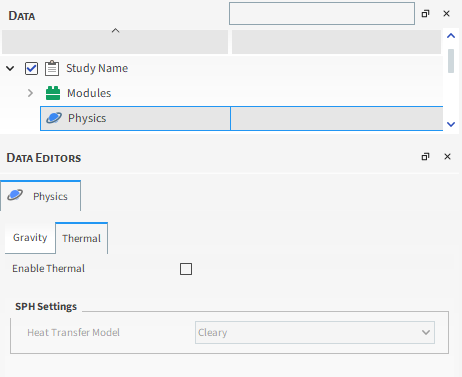
When you wish to automatically transfer FreeFlow's HTC calculations to Mechanical, when connecting the FreeFlow system to a Seady-State or a Transient Thermal using Workbench, there is no need to activate the Thermal calculations in FreeFlow's physics, as shown below:
Figure 3.123: Physics thermal tab when HTC transfer between FreeFlow and Mechanical via Workbench is used.
When this transfer is activated, a module called SPH HTC Calculator is automatically enabled in FreeFlow:
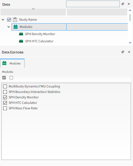
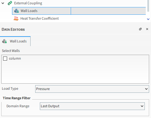
This enables another component in the External Coupling, the Heat Transfer Coefficient, which lets you assing the walls for which the HTC shall occur, a Time Range Filter for the transfer to happen and a required Reference Temperature:
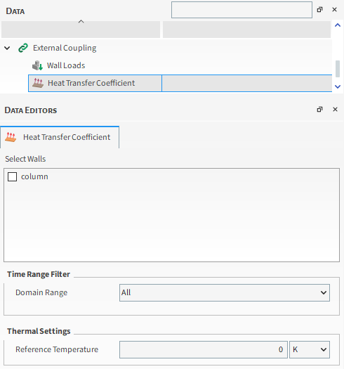
HEAT TRANSFER COEFFICIENT PARAMETERS
Use the image above and table below to help you understand how to define options for the HTC transfer.
Table 1: Heat Transfer Coefficient Parameter Definitions
|
Setting |
Description |
Range |
|---|---|---|
|
Select Walls |
Enables you to choose which geometry data will be shared during the coupled simulation. |
Turns on or off |
|
Time Range Filter |
Defines what time steps of the simulation are included in the data to be shared. The options are as follows:
|
Application Time Filter; All; Last Output; Time Range; Specify Time; After Time; Time Range Relative to Simulation End |
|
Initial |
When Time Range or After Time is chosen for Domain Range, this is the starting time to begin the time step selection. |
Any value between 0 and the final simulation time. |
|
Final |
When Time Range is chosen for Domain Range, this is the ending time to stop the time step selection. |
Any value between the Initial time and the final simulation time. |
|
At Time |
When Specific Time is chosen for Domain Range, this is the exact moment in which the time step will be selected. |
Any value between 0 and the final simulation time. |
|
Range from end |
When Time Range Relative to Simulation End is chosen for Domain Range, this is the period of time before the final simulation time in which time steps will be included in the selection. For example, when you want to include only the last X seconds of the simulation. |
Any value between 0 and the final simulation time. |
| Thermal Settings | Reference Temperature: defines the reference temperature for the HTC Calculation | Any value. |
1-WAY COUPLING WITH MECHANICAL
Ansys Products needed: Ansys FreeFlow and Ansys Mechanical.
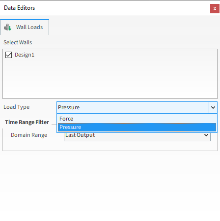
For projects coupled specifically with Ansys Mechanical, opening the Wall Loads in the Data Editors panel enables you to select which FreeFlow data items you want transferred to the Workbench connected Mechanical program.
For example, you can select which Walls you want to analyze in Mechanical, i.e, which loads are to be transferred and which load type you want between Force and Pressure.
See the image below:
You can then select the results domain of the analysis that will be exported by setting the time range.
Important: When making a 1-way coupling with Mechanical (both 1-Way HTC and 1-Way Static and Transient Structural) the connection between FreeFlow Geometry and Results to Mechanical Geometry and Setup must be done manually, instead of dragging the Mechanical system and dropping it on top of the FreeFlow one. Otherwise, the coupling may not occur properly. This process is needed because, for both 1-Way Static and Transient Structural (Forces only) and 1-Way HTC coupling between FreeFlow and Mechanical, the data from FreeFlow are automatically sent to Mechanical. For Pressure in the 1-Way Static and Transient Structural, the copy and paste between .csv files is needed.
2-WAY THERMAL COUPLING WITH MECHANICAL
Ansys Products needed: Ansys FreeFlow, Ansys Mechanical, Ansys Workbench, System Coupling and Ensight.
With this coupling it is possible to send heat from FreeFlow and receive back the temperature from Mechanical using the System Coupling.
To do this, you are able to create a coupled wall inside FreeFlow and the System Coupling will identify this walls as regions where the coupling is going to happen.
Limitations:
The coupled walls cannot have:
Motion Frame
Translation
Rotation
Mass tab
Replication tab
1- SETUP IN ANSYS FreeFlow
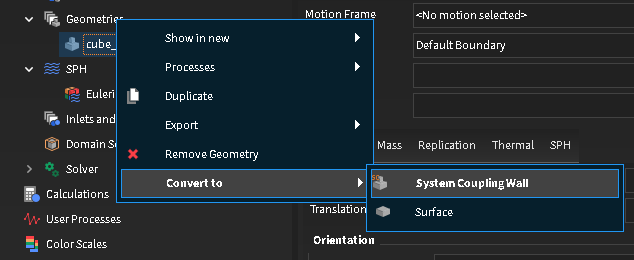
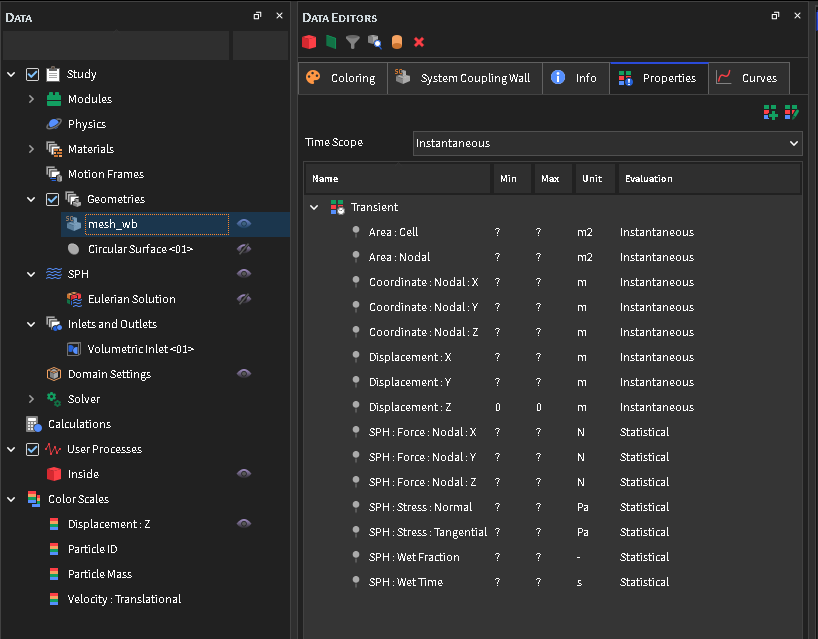
Set up your simulation as you wish, then you will have to stipulate within FreeFlow which geometry of your simulation you want to couple.
To do this, right-click on the desired geometry, then click on Convert to and then on System Coupling Wall.
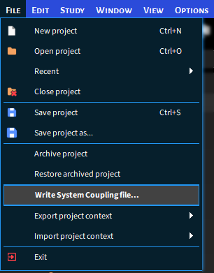
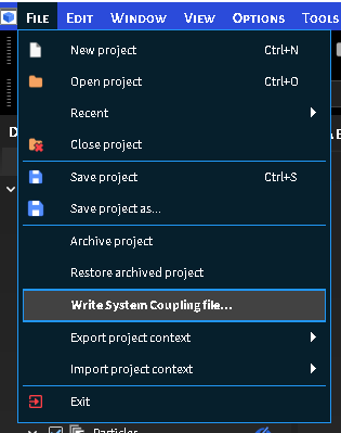
Click on File and then on Write System Coupling file. This step creates a file with information about where your FreeFlow file is for System Coupling.


2- SETUP IN ANSYS MECHANICAL
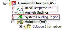
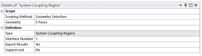
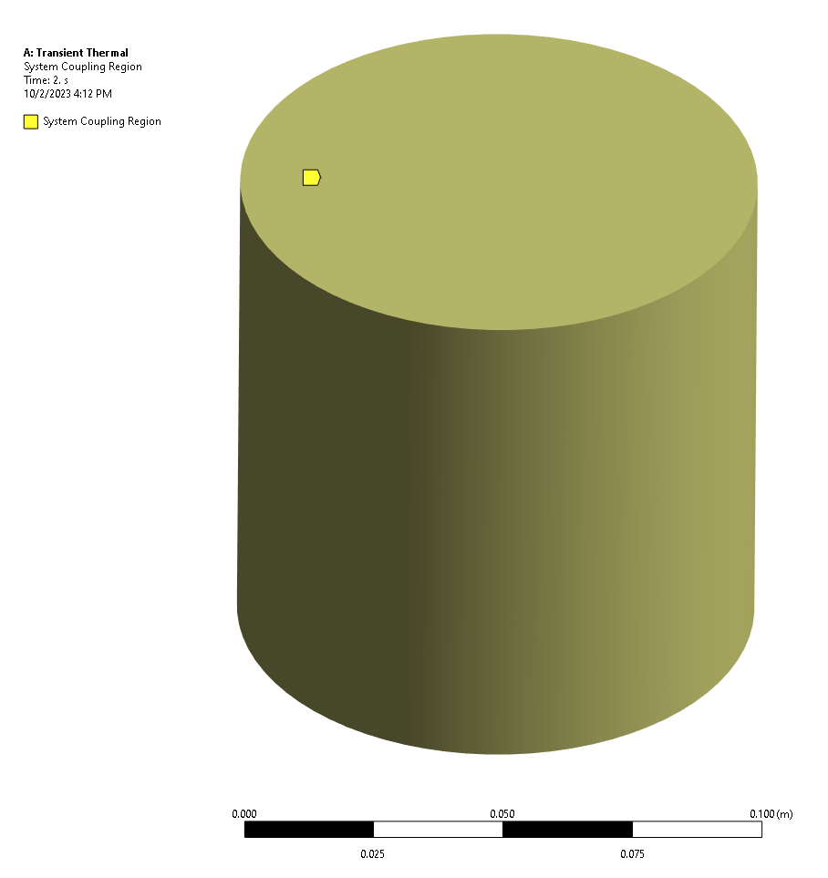
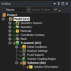
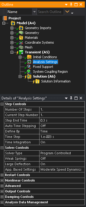
Open your project in Ansys Mechanical and set the Initial Temperature and the System Coupling Region using the Transient Thermal option.
Set the System Coupling Region, as shown in the figures below:
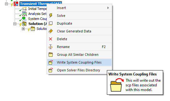
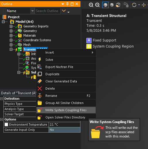
Export the System Coupling File, by right-clicking on Transient Thermal and then on Write System Coupling Files.
3- SETUP IN ANSYS WORKBENCH (TRANSIENT THERMAL)
Open your project in the Ansys Workbench and set the 2-way Thermal Coupling using the Transient Thermal option.
4- SETUP SYSTEM COUPLING
Open System Coupling and select a folder of your choice.
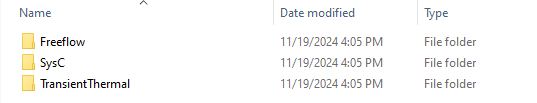
Tip: When you are doing this coupling, it is advisable to create three folders for your project, one for FreeFlow, another for Workbench and another for System Coupling.
Note: When adding the folder some Warnings will appear in the message tab, but they will be resolved as you do the setup.
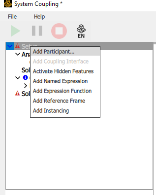
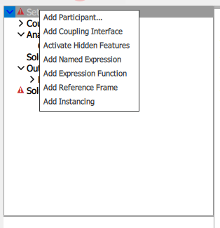
In the Data Panel, right-click Setup and then click Add Participant.
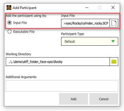
In the Add Participant window, select Input File and add the System Coupling File (.SCP) you saved from FreeFlow.
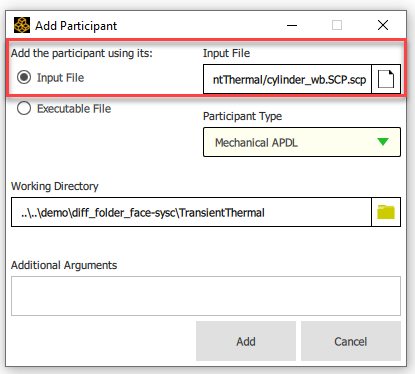
Repeat step 1, and in the Add Participant window, select Input File and add the System Coupling File (.SCP) you saved from Mechanical.
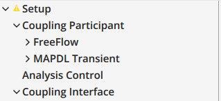
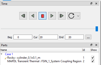
Your Data Panel must have both FreeFlow and Mechanical files:
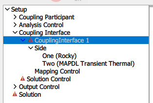
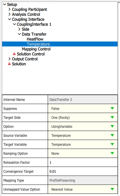
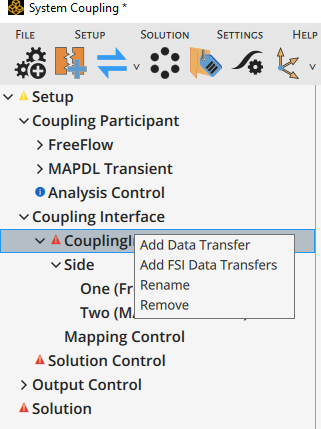
In the Data Panel, right-click Setup and then click Add Coupling Interface.
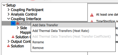
Right Click on Coupling Interface and then click on Add Data Transfer.
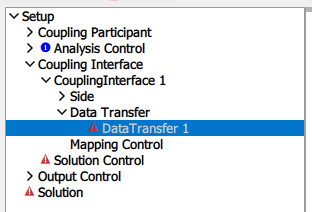
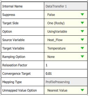
Set the Data Transfer to FreeFlow as show in the figures below:
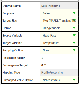
Repeat step 6, and set the Data Transfer to Mechanical as show in the figures below:
In the example below the FreeFlow Data Transfer is named as Temperature and the Mechanical Data Transfer is named as Heat Flow:
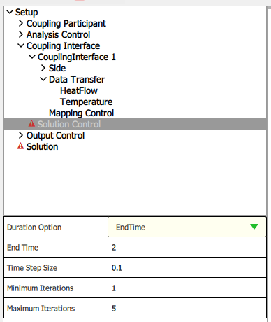
In Solution Control define the End Time and the Time Step Size.
Important: The same End Time and Time Step Size that you add in FreeFlow and Mechanical, you must add in System Coupling.
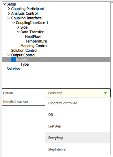
In Output Control, click on Results, and then on Type and select the Every Step option, as shown in the figure below:
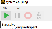
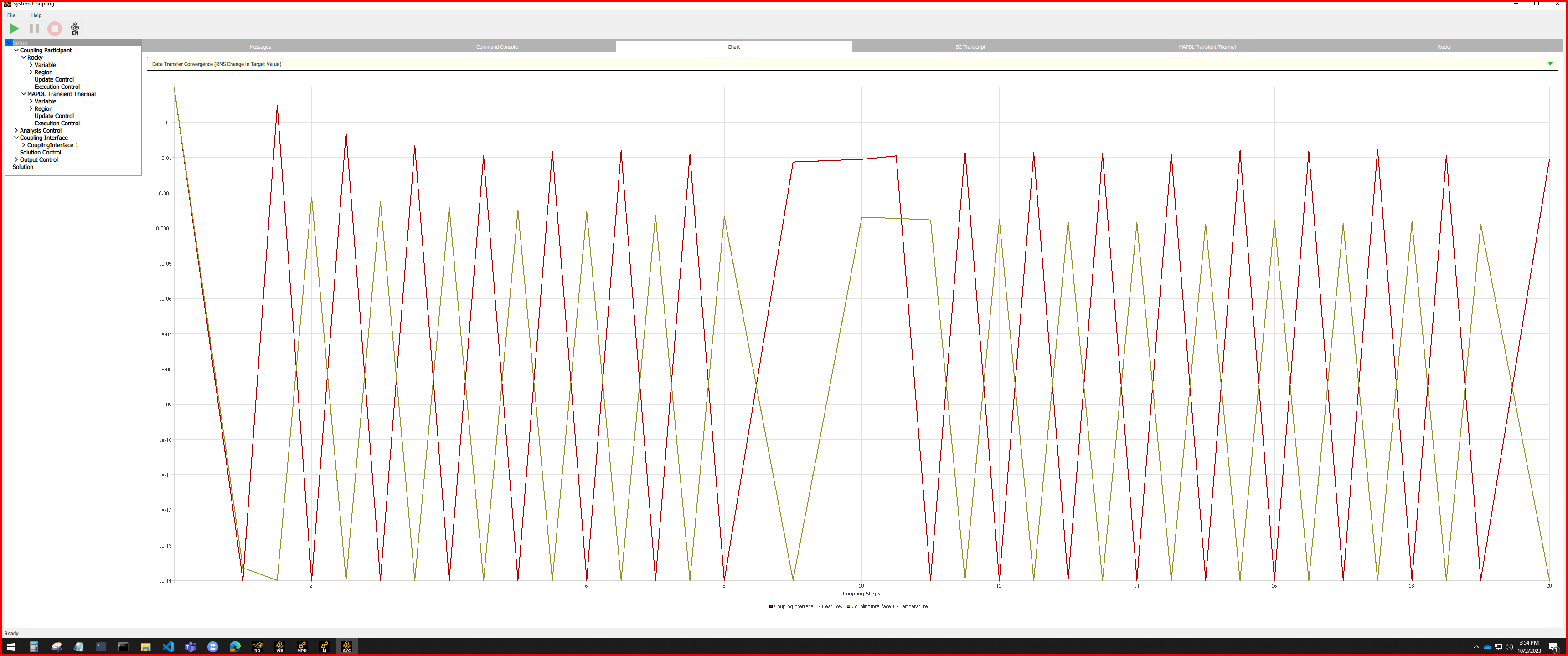
Click on Start Solve.
5- POST PROCESSING IN ENSIGHT
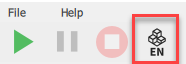
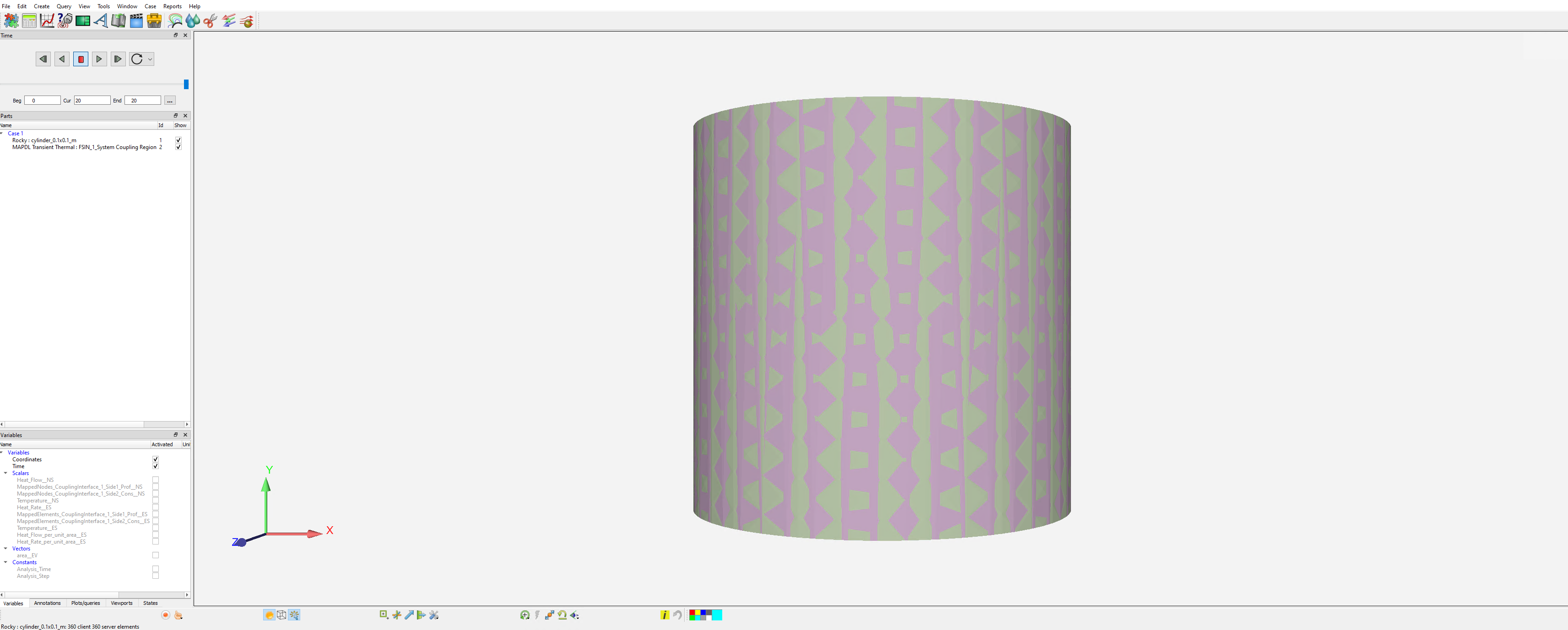
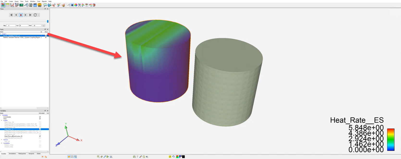
After solving your simulation, the post processing phase is carried out using the EnSight. Click on EnSight:
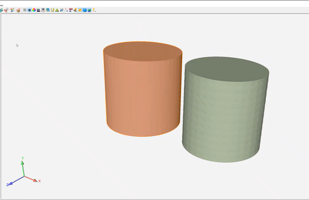
The geometries will appear in EnSight as shown in the figure below, one on top of the other, if you prefer you can separate them:
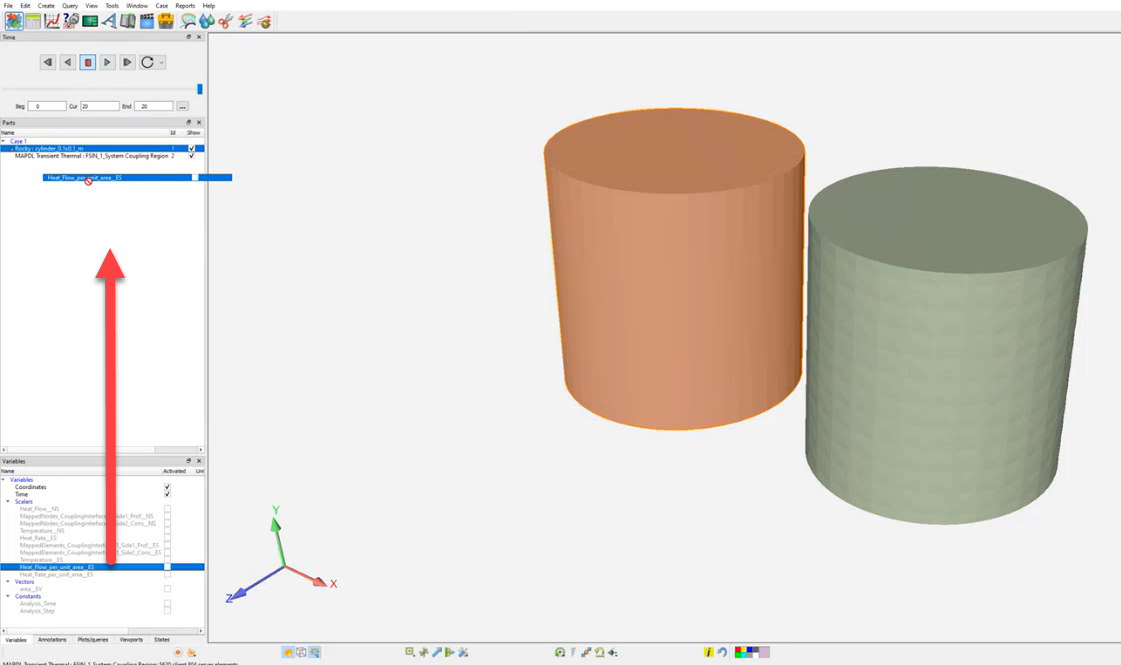
To see the results you have to drag the desired parameter to the geometry you want to see the result:
2-WAY STRUCTURAL COUPLING WITH MECHANICAL
Ansys Products needed: Ansys FreeFlow, Ansys Mechanical, Ansys Workbench, System Coupling and Ensight.
With this coupling, it is possible to send the SPH forces from FreeFlow and receive back the boundary displacement from Mechanical using the System Coupling.As the 2-Way Thermal coupling between FreeFlow and Mechanical (using the Transient Thermal one), the 2-Way Structural coupling uses the Transient Structural System inside Workbench. The main setup process is the same as already explained for the Thermal one, with just simple differences, that will be shown below.
1- SETUP IN ANSYS FreeFlow
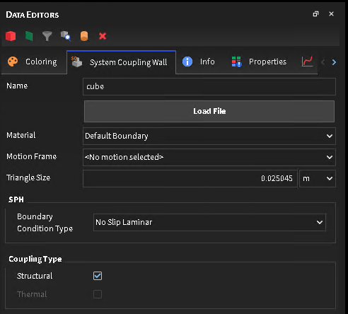
For the FreeFlow side, the first difference is that now, there are 2 Coupling Types options for the System Coupling Wall. For the 2-Way Structural Coupling, just select the Structural one. And for the 2-Way Thermal, just select the Thermal one.
The rest of FreeFlow setup, as well the Write System Coupling file is the same as 2-Way Thermal.
2- SETUP IN ANSYS MECHANICAL
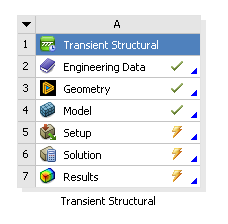
The difference from the Mechanical side is that now, the Transient Structural system for the Workbench that will be needed, as show in this image
The Model data tree setup process follows the same default Structural one, with just the System coupling regions as already described for the Thermal.
One important point here is that the Time Step inside the Analysis System, for most of the cases, will need to have a small number, as the SPH collisions will happen in a small-time fraction, and as Mechanical is an Implicit Solver, the Time Step here will need to be smaller. With the biggest time steps, Mechanical will not be able to converge, and a High Element Distortion message will be shown in the System Coupling UI.
After the setup, the System Coupling Region must be exported.
4- SETUP IN SYSTEM COUPLING
For the System Coupling side, all first steps are still the same. The only difference will be at Add Data Transfer, which now will have the Add FSI Data Transfer, which mainly will connect the forces data from FreeFlow, and send it to Mechanical.
Tip: When you are doing this coupling, it is advisable to create three folders for your project, one for FreeFlow, another for Workbench and another for System Coupling.
During the System Coupling solve process, it will be noticed that now, the Data Transfer will be the Force (FreeFlow to Mechanical) and Incremental Displacement (Mechanical to FreeFlow).
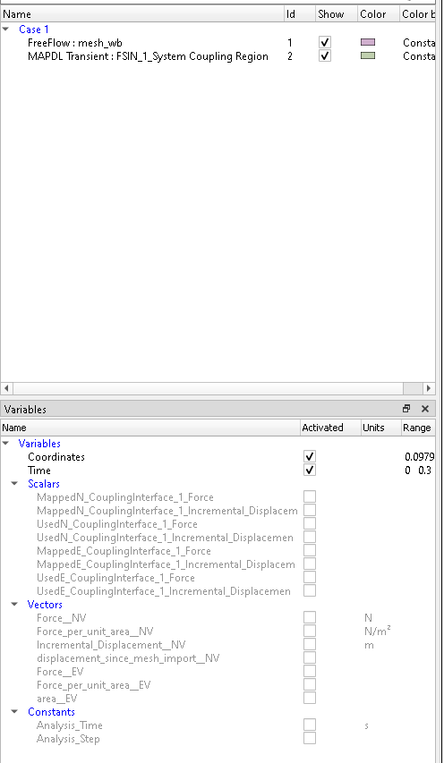
In the latest part, which is the post-processing, the two options remain: use Ensight directly from the System Coupling UI, or open FreeFlow and analyze the SPH trajectory and the Displacement results. At Ensight, new Variables are available, such as Force, Incremental Displacement, and Displacement Since Mesh Import, and for the FreeFlow side, the Displacement property will show up.
See Also:
Ansys FreeFlow can be coupled with Ansys Fluent through the SPH Point Cloud Air Drag (Beta) module. This module uses a point cloud created from Ansys Fluent simulation that gathers data from the fluid flow to interact with SPH from FreeFlow.
To download this module, you must access the Ansys Customer Portal and find FreeFlow SDK and Modules package, under Add-on Packages.
Additional info can be found at SPH Point Cloud Air Drag (Beta).
See Also:
In FreeFlow the coupling with Ansys Motion is done through a built-in FreeFlow module called Multibody Dynamics FMU Coupling.
The Ansys Motion Coupling installer will only install the FMU Export extensions for Ansys Motion. To run a coupled simulation with any FMU file, the user must enable the Multibody Dynamics FMU Coupling FreeFlow module. Another detail is that the user won't need to install the modules for each user on the same machine anymore.
Note: For Ansys Motion software and Adams, modules for these software are still needed to export the FMU files.
Similar to the FreeFlow support for the center of mass or the arrow (normal or not), that follow an internal motion frame (associated with a geometry), now both follow an external motion, as an FMU, through Multi-Body Dynamics (MBD) coupling with Ansys Motion.
For additional details regarding the Ansys Motion Coupling can be found in the Installation Guide.
See Also:
Improved integration between Ansys optiSLang and Ansys FreeFlow can boost your iterative design processes. By combining your Ansys FreeFlow cases with the robust design optimization (RDO) methods of optiSLang, processes that require multiple repeat runs - such as those for material calibration - become faster and more efficient. And when combined with the powerful parametric modeling capabilities of Ansys Workbench, you can take these efficiencies even farther.
Using the optiSLang plugin, the input parameter selection and variation for your FreeFlow projects are automatic based on sensitivity analyses and meta-modeling techniques. These automatic methods reduce the number of iterative cases that need to be run and increase the confidence with which you can adjust the interaction parameters for your calibration projects.
Important: Before you begin, ensure that the FreeFlow project you want to integrate with optiSLang has already been processed in FreeFlow and has simulation results.If you have only one license of FreeFlow, ensure that your FreeFlow program is closed, as optiSLang software will need to open it as part of the integration process.
It is possible to integrate Ansys optiSLang with Ansys FreeFlow, as shown below:
Open the Ansys optiSLang program.
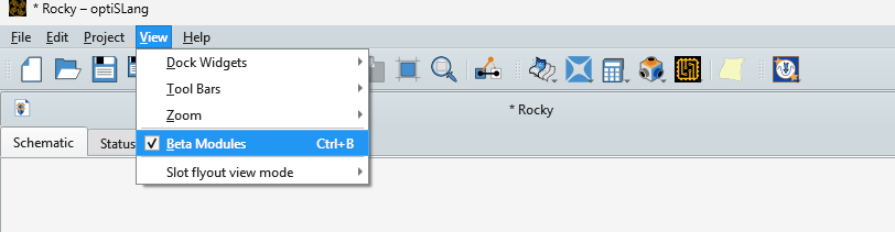
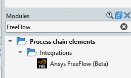
To use the Ansys FreeFlow (Beta) integrated module activate the beta modules function as illustrated in the image below:
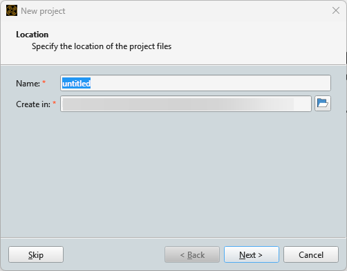
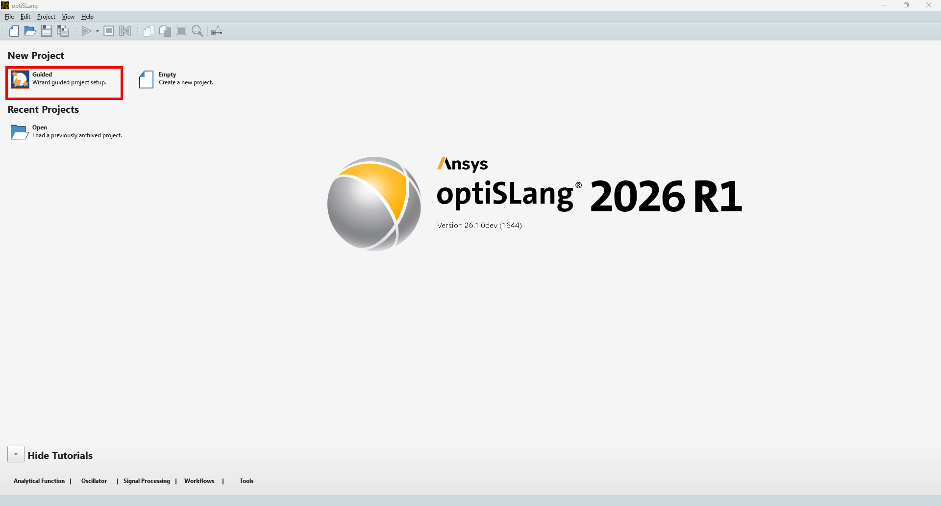
Create a new optiSLang project.
From the main Ansys optiSLang screen, under New Project, click Guided (as shown) to open the Solver Wizard.
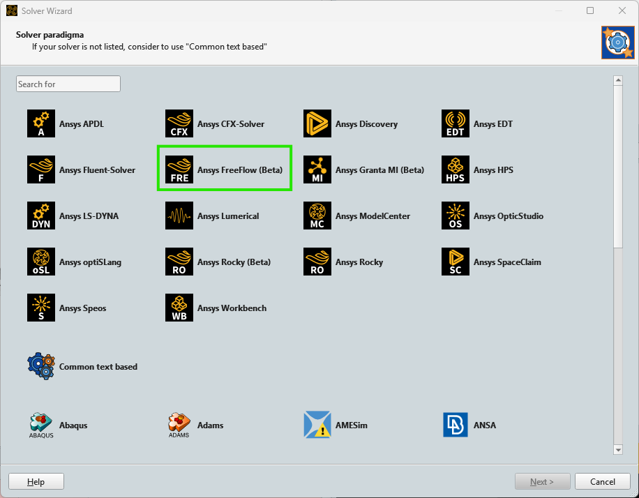
From the Solver Wizard, search for FreeFlow, and then under Interfaces, select the Ansys FreeFlow integrated module as shown below:
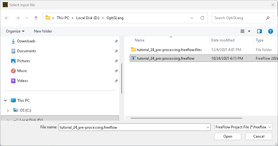
From the Select Project File dialog, navigate to Ansys FreeFlow and then select the already-processed FreeFlow project file you want to use. Click Open (as shown).
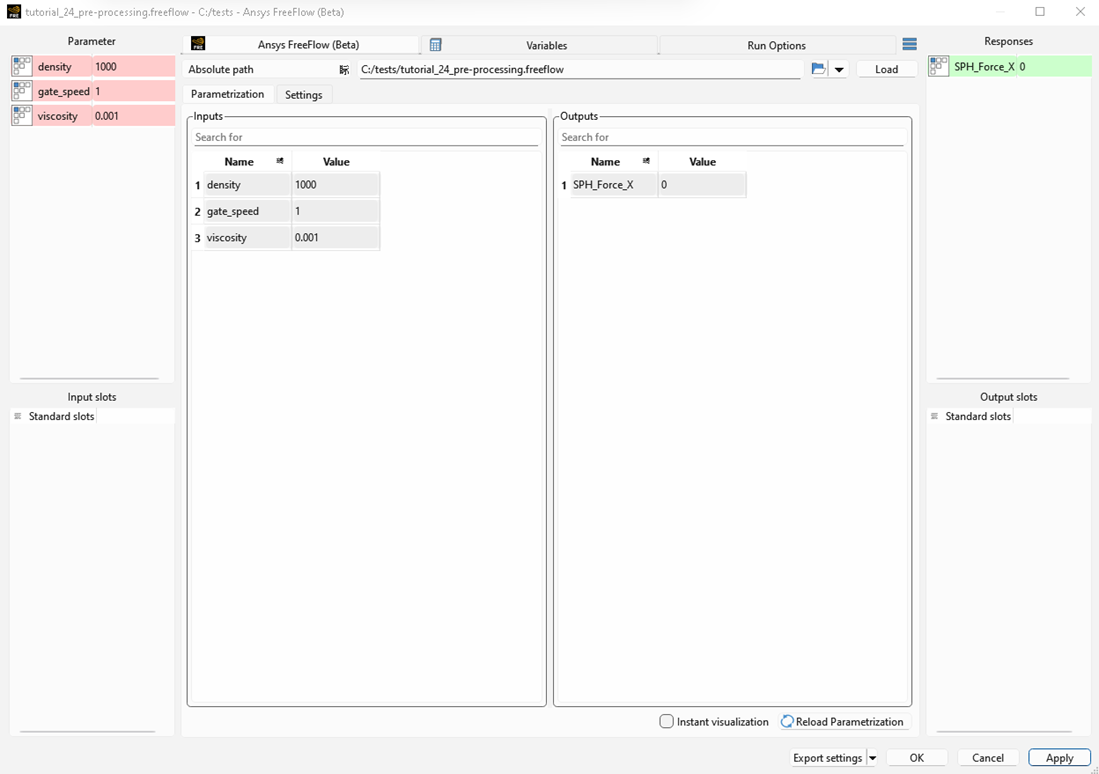
In the Ansys FreeFlow (Beta) module window, you will be able to define the solver settings, as shown in the Figure below. If you have loaded the Ansys FreeFlow (Beta) module from the “Modules” dock instead of using the Solver Wizard, you will be required to enter the FreeFlow project path.
If your FreeFlow project has Input parameters, they will be listed under the Inputs field, and you can choose which ones to use by dragging and dropping them to the Parameter field, as shown in the Figure above.
Similarly, the output parameters can be selected from the Output to the Response field.
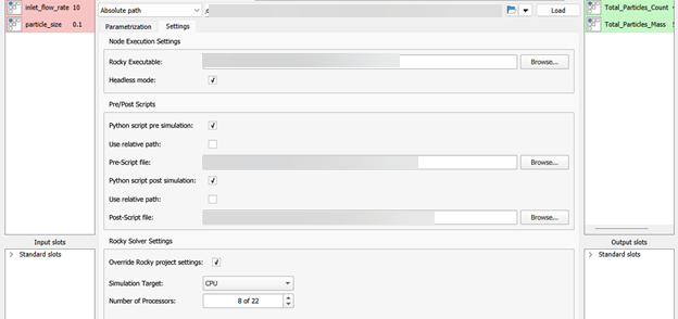
In the "Settings" tab, you can set some options for node execution, namely:
Changing the FreeFlow executable (by default, the plugin will use the FreeFlow executable in the ANSYS folder of the same version of optiSLang, if found).
By default, FreeFlow will run in headless mode, but you can deactivate this option to have FreeFlow GUI launched for each design point during optiSLang executions.
To define a script to be run inside FreeFlow before the simulation is executed ("Pre-Script file").
To define a script to be run inside FreeFlow after the simulation is executed ("Post-Script file").
Override FreeFlow Solver settings related to the "Simulation Target" (CPU/GPU).
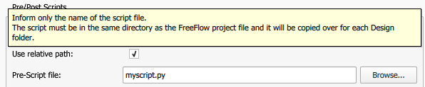
Note: If the Pre/Post scripts are set to "use relative path," only the name of the file must be provided; it must be in the same directory as the .FreeFlow file, and it will be copied to each Design folder (as is informed by a tooltip when hovering this setting in the UI).
The Ansys FreeFlow (Beta) module will be available in the Schematic view. The parameters can be edited at any time by double-clicking the FreeFlow node.
Note: By default, optiSLang creates .py files for this purpose in the same folder as the FreeFlow project you selected earlier. After optiSLang loads the input/output variables, FreeFlow will launch and you will receive a confirmation message.
Tip: For more information about using optiSLang, refer to the Ansys/Dynardo optiSLang User Documentation.