8.1. Function Expressions

A Function Expression represents a formula. This entity can be used in the formulation of a force or motion, and for measurement of displacement, velocity, acceleration, and force between several markers in a subsystem.

8.1.1. Various Functions

Various intrinsic functions are supported in a Function Expression as shown in the table below. The resultant value of these intrinsic functions is a scalar.

Figure 8.1: Intrinsic functions in Function expression

Category	Description
Math Functions	Use to set functions defined at the C/C++ math library.
Simulation Constants	Use to set variables with an intrinsic keyword.
Displacement Functions	Use to calculate the position or angle between the markers.
Velocity Functions	Use to calculate the translational velocity or angular velocity between the markers.
Acceleration Functions	Use to calculate the translational acceleration or angular acceleration between the markers.
Generic Force Functions	Use to calculate the force or torque between two markers.
Contact Functions	Use to calculate a value related to the specified contact.
System Element Functions	Use to calculate the value of equations.
Arithmetic IF Functions	Use to operate a logical function.
Interpolation Functions	Use to calculate the value from the specified spline.
Predefined Functions	Use to set functions defined at the Motion solver.
Interface Parameters and Sub-Entity Functions	Use to calculate a variable for co-simulation or array.

8.1.2. Simulation Constants

Simulation Constants are mathematical constants and intrinsic keywords as shown in the table below.

Figure 8.2: Simulation Constants

Functions	Description
DTOR	Definition	Conversion factor from degree to radians.
DTOR	Value	0.017453…. This value is equal to PI/180.
PI	Definition	Mathematical constant equal to a circle's circumference divided by its diameter.
PI	Value	3.141592…. This value is equal to ACOS(-1).
RTOD	Definition	Conversion factor from radians to degree.
RTOD	Value	57.29577…. This value is equal to 180/PI.
TIME	Definition	Simulation time
TIME	Value	Real variable, equal to the simulation time.

8.1.3. Math Functions

Math functions which are supported from the C/C++ math library are shown below:

Figure 8.3: Math functions

Functions	Description
ABS(E1)	Definition	Use to compute the absolute value of E1.
	Input (E1)	Real
	Return Value	Real ≥ 0
	Example	ABS(-1.5) = 1.5
ACOS(E1)	Definition	Use to compute the arc-cosine of E1.
	Input (E1)	-1 ≤ Real ≤ 1. If the input value is greater than 1 or less than -1, it will be limited 1 or -1, respectively.
	Return Value	0 ≤ Real < PI in Radian
	Example	ACOS(0.5) = PI/3
AINT(E1)	Definition	Use to truncate E1 to the whole number part.
	Input (E1)	Real
	Return Value	Integer. If the magnitude of E1 is less than 1, then AINT(E1) returns 0. If the magnitude is equal to or greater than 1, then it returns the largest whole number that does not exceed its magnitude. The sign is the same as the sign of E1.
	Example	AINT(-1.5678) = -1, AINT(0.17) = 0
ANINT(E1)	Definition	Use to round E1 to the nearest whole number.
	Input (E1)	Real
	Return Value	Integer. If E1 is greater than 0, then ANINT(X) returns AINT(E1+0.5). If E1 is less than or equal to 0, then return AINT(E1-0.5).
	Example	ANINT(0.4) = 0, ANINT(-1.9) = -2
ASIN(E1)	Definition	Use to compute the arcsine of E1.
	Input (E1)	-1 ≤ Real ≤ 1. If the input value is greater than 1 or less than -1, it will be limited 1 or -1, respectively.
	Return Value	-PI/2 ≤ Real ≤ PI/2 in Radians
	Example	ASIN(0.5) = PI/6
ATAN(E1)	Definition	Use to compute the arctangent of E1.
	Input (E1)	Real
	Return Value	-PI/2 ≤ Real ≤ PI/2 in Radians
	Example	ATAN(1.0) = PI/4
ATAN2(E1,E2)	Definition	Use to compute the arctangent of E2/E1.
	Input (E1,E2)	Real
	Return Value	-PI < Real ≤ PI in Radian. The return value can be computed under several conditions as follows. 1) E1 > 0 → ATAN(E2/E1) 2) E1 < 0 & E2 ≥ 0 → ATAN(E2/E1) + PI 3) E1 < 0 & E2 ≤ 0 → ATAN(E2/E1) - PI 4) E1 = 0 & E2 > 0 → PI/2 5) E1 = 0 & E2 < 0 → -PI/2 6) E1 = 0 & E2 = 0 → 0
	Example	ATAN2(1.0,-1.0) = -PI/4, ATAN2(-1.0,1.0) = 3*PI/4
CEIL(E1)	Definition	Use to return the least integer greater than or equal to E1.
	Input (E1)	Real
	Return Value	Integer
	Example	CEIL(0.4) = 1, CEIL(-0.9) = 0
COS(E1)	Definition	Use to compute the cosine of E1.
	Input (E1)	Real in Radians
	Return Value	Real
	Example	COS(PI/3) = 0.5
COSH(E1)	Definition	Use to compute the hyperbolic cosine of E1.
	Input (E1)	Real in Radians
	Return Value	Real
	Example	COSH(PI/18) = 1.01526957
DIM(E1,E2)	Definition	Use to compute the difference E1-E2 if the result is positive. Otherwise returns zero.
	Input (E1,E2)	Real
	Return Value	Real ≥ 0
	Example	DIM(2,1) = 1, DIM(1,2) = 0
DIVISION(E1,E2)	Definition	Use to compute the division of E1 by E2, avoiding the division by 0 problem.
	Input (E1,E2)	Real
	Return Value	Real. The return value can be computed under several conditions as follows. 1) E2 = 0 → 0 2) E2 != 0 → E1/E2
	Example	DIVISION(10,4) = 2.5
EXP(E1)	Definition	Use to compute the base e exponential of E1.
	Input (E1)	Real
	Return Value	Real
	Example	EXP(1.0) = e (Euler's number)
FLOOR(E1)	Definition	Use to return the greatest integer less than or equal to E1.
	Input (E1)	Real
	Return Value	Integer
	Example	FLOOR(0.4) = 0, FLOOR(-0.9) = -1
LOG(E1)	Definition	Use to compute the natural (base e) logarithm of E1.
	Input (E1)	Real > 0
	Return Value	Real
	Example	LOG(2.7182818) = 1.0
LOG10(E1)	Definition	Use to compute the base 10 logarithm of E1.
	Input (E1)	Real > 0
	Return Value	Real
	Example	LOG(100.0) = 2.0
MAX(E1,E2)	Definition	Use to return the maximum value of E1 and E2.
	Input (E1,E2)	Real
	Return Value	Real
	Example	MAX(1,2) = 2
MIN(E1,E2)	Definition	Use to return the minimum value of E1 and E2.
	Input (E1,E2)	Real
	Return Value	Real
	Example	MIN(1,2) = 1
MOD(E1,E2)	Definition	Use to computes the remainder of the division of E1 by E2.
	Input (E1,E2)	Real. E2 must be not equal to zero.
	Return Value	Real. The return value can be calculated as follows. E1 - INT(E1/E2) * E2.
	Example	MOD(9,4) = 1
POW(E1,E2)	Definition	Use to computes E1 raised to the power of E2.
	Input (E1,E2)	Real. E1 must be not equal to zero.
	Return Value	Real. The return value can be computed under several conditions as follows. 1) E1 > 0 → E1^E2 2) E1 = 0 & E2 > 0 → 0 3) E1 = 0 & E2 = 0 → 1 4) E1 = 0 & E2 < 0 → 0 5) E1 < 0 & E2 is an integer number. → E1^E2 6) E1 < 0 & E2 has a finite decimal. → 0 For 4) case and 6) cases, the return value is not calculated but actually Motion solver returns zero value.
	Example	POW(2,4) = 16
RAND(E1,E2)	Definition	Use to returns a pseudo-random number from a uniform distribution between E1 and E2.
	Input (E1,E2)	Real. E2 must be greater than E1.
	Return Value	Real
	Example	RAND(6,9) = 6, 7, 8 or 9
SIGN(E1,E2)	Definition	Use to return the value of E1 with the sign of E2.
	Input (E1,E2)	Real
	Return Value	Real
	Example	SIGN(7,-1) = -7, SIGN(-7,-1) = -7, SIGN(-7,1) = 7
SIN(E1)	Definition	Use to compute the sine of E1.
	Input (E1)	Real in Radians
	Return Value	Real
	Example	SIN(PI/6) = 0.5
SINH(E1)	Definition	Use to compute the hyperbolic sine of E1.
	Input (E1)	Real in Radians
	Return Value	Real
	Example	SINH(PI/18) = 0.17542037
SQRT(E1)	Definition	Use to compute the square root of E1.
	Input (E1)	Real ≥ 0
	Return Value	Real ≥ 0
	Example	SQRT(4) = 2
TAN(E1)	Definition	Use to compute the tangent of E1.
	Input (E1)	Real in Radian. E1 must be not equal to (2N-1)*PI/2.
	Return Value	Real
	Example	TAN(PI/4) = 1.0
TANH(E1)	Definition	Use to compute the hyperbolic tangent of E1.
	Input (E1)	Real in Radians
	Return Value	Real
	Example	TANH(PI/18) = 0.172782

Note: For cases of infinite value, the Motion solver returns zero.

If division by zero occurs, a warning message will be printed in the *.msg file and the result of function expression will be treated as 0. In this case, the solution may differ from versions prior to 2023 R2. To avoid this problem, use the DIVISION function.

8.1.4. Displacement Functions

Displacement Functions can be defined as shown in the table below. For each function, if the base and reference markers are not defined, they will be automatically set to the inertia reference marker. The position and orientation of the inertia reference marker are the zero vector and the identity matrix, respectively. The reference marker and base marker can be defined as the same marker, if required.

Figure 8.4: Displacement Functions

Functions	Description
DM(E1,{E2})	Definition	The magnitude of the relative position between the markers.
	Input (E1,E2)	E1 and E2 are the names or argument IDs of the action and base markers.
	Return Value	From Equation 2–65, the magnitude of the vector can be returned as follows: .
	Example	DM(p1), DM(p1,p2)
DX(E1,{E2},{E3})	Definition	The x-component of the relative position between the markers.
	Input (E1,E2, E3)	E1, E2 and E3 are the names or argument IDs of the action, base and reference markers.
	Return Value	From Equation 2–66, the x-component of the vector can be returned as follows. ,where .
	Example	DX(p1), DX(p1,p2), DX(p1,p2,p2), DX(p1,p2,p3)
DY(E1,{E2},{E3})	Definition	The y-component of the relative position between the markers.
	Input (E1,E2, E3)	E1, E2 and E3 are the names or argument IDs of the action, base and reference markers.
	Return Value	From Equation 2–66, the y-component of the vector can be returned as follows. ,where .
	Example	DY(p1), DY(p1,p2), DY(p1,p2,p2), DY(p1,p2,p3)
DZ(E1,{E2},{E3})	Definition	The z-component of the relative position between the markers.
	Input (E1,E2, E3)	E1, E2 and E3 are the names or argument IDs of the action, base and reference markers.
	Return Value	From Equation 2–66, the z-component of the vector can be returned as follows. ,where .
	Example	DZ(p1), DZ(p1,p2), DZ(p1,p2,p2), DZ(p1,p2,p3)
AX(E1,{E2})	Definition	The relative angle with respect to the x-axis of the base marker.
	Input (E1,E2)	E1 and E2 are the names or argument IDs of the action and base markers.
	Return Value	The angle in Equation 2–82 will be returned in radians.
	Example	AX(p1), AX(p1,p2)
AY(E1,{E2})	Definition	The relative angle with respect to the y-axis of the base marker.
	Input (E1,E2)	E1 and E2 are the names or argument IDs of the action and base markers.
	Return Value	The angle in Equation 2–83 will be returned in radians.
	Example	AY(p1), AY(p1,p2)
AZ(E1,{E2})	Definition	The relative angle with respect to the z-axis of the base marker.
	Input (E1,E2)	E1 and E2 are the names or argument IDs of the action and base markers.
	Return Value	The angle in Equation 2–84 will be returned in radians.
	Example	AZ(p1), AZ(p1,p2)
PSI(E1,{E2})	Definition	The first rotation angle from ZXZ Euler angle.
	Input (E1,E2)	E1 and E2 are the names or argument IDs of the action and base markers.
	Return Value	The angle in Equation 2–76 will be returned in radians.
	Example	PSI(p1), PSI(p1,p2)
THETA(E1,{E2})	Definition	The second rotation angle from ZXZ Euler angle.
	Input (E1,E2)	E1 and E2 are the names or argument IDs of the action and base markers.
	Return Value	The angle in Equation 2–77 will be returned in radians.
	Example	THETA(p1), THETA(p1,p2)
PHI(E1,{E2})	Definition	The third rotation angle from ZXZ Euler angle.
	Input (E1,E2)	E1 and E2 are the names or argument IDs of the action and base markers.
	Return Value	The angle in Equation 2–78 will be returned in radians.
	Example	PHI(p1), PHI(p1,p2)
YAW(E1,{E2})	Definition	The first rotation angle from ZYX Euler angle. In the general sense, this can represent a relative angle between two markers with respect to the z-axis of the base marker.
	Input (E1,E2)	E1 and E2 are the names or argument IDs of the action and base markers.
	Return Value	The angle in Equation 2–79 will be returned in radians.
	Example	YAW(p1), YAW(p1,p2)
PITCH(E1,{E2})	Definition	The second rotation angle from ZYX Euler angle. In the general sense, this can represent a relative angle between two markers with respect to the y-axis of the base marker.
	Input (E1,E2)	E1 and E2 are the names or argument IDs of the action and base markers.
	Return Value	The angle in Equation 2–80 will be returned in radians.
	Example	PITCH(p1), PITCH(p1,p2)
ROLL(E1,{E2})	Definition	The third rotation angle from ZYX Euler angle. In the general sense, this can represent a relative angle between two markers with respect to the x-axis of the base marker.
	Input (E1,E2)	E1 and E2 are the names or argument IDs of the action and base markers.
	Return Value	The angle in Equation 2–81 will be returned in radians.
	Example	ROLL(p1), ROLL(p1,p2)

8.1.5. Velocity Functions

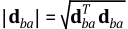
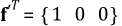
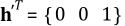
Velocity Functions can be defined as shown in the table below. In each function, if the base and reference markers are not defined, they will be automatically set to the inertia reference marker. The position and velocities of the inertia reference marker are zero vectors and its orientation is defined as the identity matrix. The reference marker and base marker can be defined as the same marker, if required.

Figure 8.5: Velocity Functions

Functions	Description
VM(E1,{E2})	Definition	The magnitude of the relative velocity between the markers.
	Input (E1,E2)	E1 and E2 are the names or argument IDs of the action and base markers.
	Return Value	From Equation 2–92, the magnitude of the vector can be returned as follows.
	Example	VM(p1), VM(p1,p2)
VR(E1,{E2})	Definition	The relative velocity in the direction of the relative displacement between two markers.
	Input (E1,E2)	E1 and E2 are the names or argument IDs of the action and base markers.
	Return Value	The relative velocity in Equation 2–101 will be returned.
	Example	VR(p1), VR(p1,p2)
VX(E1,{E2},{E3})	Definition	The x-component of the relative velocity between the markers.
	Input (E1,E2, E3)	E1, E2 and E3 are the names or argument IDs of the action, base and reference markers.
	Return Value	From ????, the x-component of the vector can be returned as follows. , where ,where .
	Example	VX(p1), VX(p1,p2), VX(p1,p2,p2), VX(p1,p2,p3)
VY(E1,{E2},{E3})	Definition	The y-component of the relative velocity between the markers.
	Input (E1,E2, E3)	E1, E2 and E3 are the names or argument IDs of the action, base and reference markers.
	Return Value	From ????, the y-component of the vector can be returned as follows. ,where .
	Example	VY(p1), VY(p1,p2), VY(p1,p2,p2), VY(p1,p2,p3)
VZ(E1,{E2},{E3})	Definition	The z-component of the relative velocity between the markers.
	Input (E1,E2, E3)	E1, E2 and E3 are the names or argument IDs of the action, base and reference markers.
	Return Value	From ????, the z-component of the vector can be returned as follows. ,where .
	Example	VZ(p1), VZ(p1,p2), VZ(p1,p2,p2), VZ(p1,p2,p3)
WM(E1,{E2})	Definition	The magnitude of the relative angular velocity between the markers.
	Input (E1,E2)	E1 and E2 are the names or argument IDs of the action and base markers.
	Return Value	From Equation 2–102, the magnitude of the vector can be returned as follows.
	Example	WM(p1), WM(p1,p2)
WX(E1,{E2},{E3})	Definition	The x-component of the relative angular velocity between the markers.
	Input (E1,E2, E3)	E1, E2 and E3 are the names or argument IDs of the action, base and reference markers.
	Return Value	From Equation 2–103, the x-component of the vector can be returned as follows. , where .
	Example	WX(p1), WX(p1,p2), WX(p1,p2,p2), WX(p1,p2,p3)
WY(E1,{E2},{E3})	Definition	The y-component of the relative angular velocity between the markers.
	Input (E1,E2, E3)	E1, E2 and E3 are the names or argument IDs of the action, base and reference markers.
	Return Value	From Equation 2–103, the y-component of the vector can be returned as follows. , where .
	Example	WY(p1), WY(p1,p2), WY(p1,p2,p2), WY(p1,p2,p3)
WZ(E1,{E2},{E3})	Definition	The z-component of the relative angular velocity between the markers.
	Input (E1,E2, E3)	E1, E2 and E3 are the names or argument IDs of the action, base and reference markers.
	Return Value	From Equation 2–103, the z-component of the vector can be returned as follows. , where .
	Example	WZ(p1), WZ(p1,p2), WZ(p1,p2,p2), WZ(p1,p2,p3)

8.1.6. Acceleration Functions

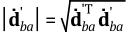
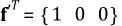
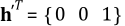
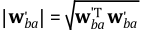
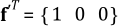
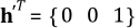
Acceleration Functions can be defined as shown in the table below. For each function, if the base and reference markers are not defined, they will be automatically set to the inertia reference marker. The accelerations of the inertia reference marker are zero vectors and its orientation is defined as the identity matrix. The reference marker and base marker can be defined as the same marker, if required.

Figure 8.6: Acceleration Functions

Functions	Description
ACCM(E1,{E2})	Definition	The magnitude of the relative acceleration between the markers.
	Input (E1,E2)	E1 and E2 are the names or argument IDs of the action and base markers.
	Return Value	From Equation 2–111, the magnitude of the vector can be returned as follows.
	Example	ACCM(p1), ACCM(p1,p2)
ACCX(E1,{E2},{E3})	Definition	The x-component of the relative acceleration between the markers.
	Input (E1,E2, E3)	E1, E2 and E3 are the names or argument IDs of the action, base and reference markers.
	Return Value	From Equation 2–112, the x-component of the vector can be returned as follows. , where .
	Example	ACCX(p1), ACCX(p1,p2), ACCX(p1,p2,p2), ACCX(p1,p2,p3)
ACCY(E1,{E2},{E3})	Definition	The y-component of the relative acceleration between the markers.
	Input (E1,E2, E3)	E1, E2 and E3 are the names or argument IDs of the action, base and reference markers.
	Return Value	From Equation 2–112, the y-component of the vector can be returned as follows. , where .
	Example	ACCY(p1), ACCY(p1,p2), ACCY(p1,p2,p2), ACCY(p1,p2,p3)
ACCZ(E1,{E2},{E3})	Definition	The z-component of the relative acceleration between the markers.
	Input (E1,E2, E3)	E1, E2 and E3 are the names or argument IDs of the action, base and reference markers.
	Return Value	From Equation 2–112, the z-component of the vector can be returned as follows. ,where .
	Example	ACCZ(p1), ACCZ(p1,p2), ACCZ(p1,p2,p2), ACCZ(p1,p2,p3)
WDTM(E1,{E2})	Definition	The magnitude of the relative angular acceleration between the markers.
	Input (E1,E2)	E1 and E2 are the names or argument IDs of the action and base markers.
	Return Value	From Equation 2–120, the magnitude of the vector can be returned as follows.
	Example	WDTM(p1), WDTM(p1,p2)
WDTX(E1,{E2},{E3})	Definition	The x-component of the relative angular acceleration between the markers.
	Input (E1,E2, E3)	E1, E2 and E3 are the names or argument IDs of the action, base and reference markers.
	Return Value	From Equation 2–121, the x-component of the vector can be returned as follows. , where .
	Example	WDTX(p1), WDTX(p1,p2), WDTX(p1,p2,p2), WDTX(p1,p2,p3)
WDTY(E1,{E2},{E3})	Definition	The y-component of the relative angular acceleration between the markers.
	Input (E1,E2, E3)	E1, E2 and E3 are the names or argument IDs of the action, base and reference markers.
	Return Value	From Equation 2–121, the y-component of the vector can be returned as follows. , where .
	Example	WDTY(p1), WDTY(p1,p2), WDTY(p1,p2,p2), WDTY(p1,p2,p3)
WDTZ(E1,{E2},{E3})	Definition	The z-component of the relative angular acceleration between the markers.
	Input (E1,E2, E3)	E1, E2 and E3 are the names or argument IDs of the action, base and reference markers.
	Return Value	From Equation 2–121, the z-component of the vector can be returned as follows. , where .
	Example	WDTZ(p1), WDTZ(p1,p2), WDTZ(p1,p2,p2), WDTZ(p1,p2,p3)

8.1.7. Generic Force Functions

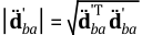
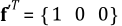
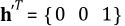
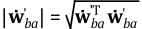
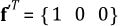
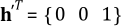
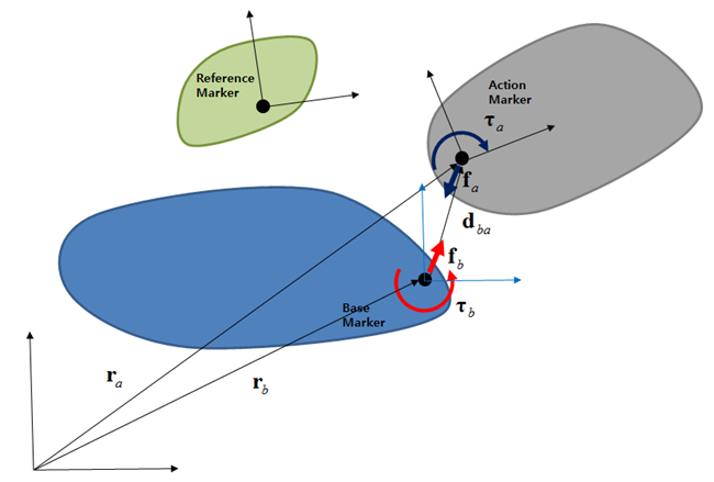
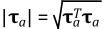
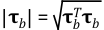
Generic Force Functions are used to measure a force or torque generated from Force and Joint entities. The markers used to define the function must be the markers used when defining the Force or Joint entity. So, if the action marker of the function is the action marker of the entity, the base marker of the function must be the base marker of the entity. In this case, the returned force or torque from the function is the force or torque applied to the action marker of the entity and they can be expressed as f_a and τ_a as shown in the figure below. Their definitions have been introduced in the documentation sections for the corresponding entity.

Figure 8.7: Kinematics for force functions

If the force or torque is measured in a reference frame, the resultant force or torque can be calculated as follows.

(8–1)

(8–2)

where A_r is the orientation matrix of the reference marker.

If the action marker of the function is the base marker of the entity, the base marker of the function must be the action marker of the entity. In this case, the returned force or torque from the function is the reaction force or torque at the base marker of the entity and can be calculated from the following equations.

(8–3)

(8–4)

If the force or torque is measured in a reference frame, the resultant force or torque can be calculated as follows.

(8–5)

(8–6)

The generic force functions can be defined as shown in the table below. 1) refers to when the retuned value is the applied force or torque and 2) refers to when the returned value is the reaction force or torque. In each function, if the reference marker is not defined, it will be automatically set to the inertia reference marker. The orientation of the inertia reference marker is defined as the identity matrix.

Figure 8.8: Generic Force Functions

Functions	Description
FM(E1,E2)	Definition	The magnitude of the force between the markers.
	Input (E1,E2)	E1 and E2 are the names or argument IDs of the action and base markers.
	Return Value	From Equation 8–3, the magnitude of the force can be returned as follows.
	Example	FM(p1,p2)
FX(E1,E2,{E3})	Definition	The x-component of the force between the markers.
	Input (E1,E2, E3)	E1, E2 and E3 are the names or argument IDs of the action, base and reference markers.
	Return Value	From Equation 8–1 and Equation 8–5, the x-component of the vector can be returned as follows. 1) 2) where .
	Example	FX(p1,p2), FX(p1,p2,p2), FX(p1,p2,p3)
FY(E1,E2,{E3})	Definition	The y-component of the force between the markers.
	Input (E1,E2, E3)	E1, E2 and E3 are the names or argument IDs of the action, base and reference markers.
	Return Value	From Equation 8–1 and Equation 8–5, the y-component of the vector can be returned as follows. 1) 2) where .
	Example	FY(p1,p2), FY(p1,p2,p2), FY(p1,p2,p3)
FZ(E1,E2,{E3})	Definition	The z-component of the force between the markers.
	Input (E1,E2, E3)	E1, E2 and E3 are the names or argument IDs of the action, base and reference markers.
	Return Value	From Equation 8–1 and Equation 8–5, the z-component of the vector can be returned as follows. 1) 2) where .
	Example	FZ(p1,p2), FZ(p1,p2,p2), FZ(p1,p2,p3)
TM(E1,E2)	Definition	The magnitude of the torque between the markers.
	Input (E1,E2)	E1 and E2 are the names or argument IDs of the action and base markers.
	Return Value	From Equation 8–4, the magnitude of the torque can be returned as follows. 1) 2)
	Example	TM(p1), TM(p1,p2)
TX(E1,E2,{E3})	Definition	The x-component of the torque between the markers.
	Input (E1,E2, E3)	E1, E2 and E3 are the names or argument IDs of the action, base and reference markers.
	Return Value	From Equation 8–2 and Equation 8–6, the x-component of the vector can be returned as follows. 1) 2) where .
	Example	TX(p1), TX(p1,p2), TX(p1,p2,p2), TX(p1,p2,p3)
TY(E1,E2,{E3})	Definition	The y-component of the torque between the markers.
	Input (E1,E2, E3)	E1, E2 and E3 are the names or argument IDs of the action, base and reference markers.
	Return Value	From Equation 8–2 and Equation 8–6, the y-component of the vector can be returned as follows. 1) 2) where .
	Example	TY(p1), TY(p1,p2), TY(p1,p2,p2), TY(p1,p2,p3)
TZ(E1,E2,{E3})	Definition	The z-component of the torque between the markers.
	Input (E1,E2, E3)	E1, E2 and E3 are the names or argument IDs of the action, base and reference markers.
	Return Value	From Equation 8–2 and Equation 8–6, the z-component of the vector can be returned as follows. 1) 2) where .
	Example	TZ(p1), TZ(p1,p2), TZ(p1,p2,p2), TZ(p1,p2,p3)

8.1.8. Contact Functions

Contact Functions are used to get results such as force, torque, penetration, or tangential velocity reported by Contact entities.

Contact Functions support General Contact, Rigid to Rigid 3D Contact (RTR3D Contact), Flex to Rigid 3D Contact (FTR3D Contact), Flex to Flex 3D Contact (FTF3D Contact), FE Tie Contact and EasyFlex Tie Contact.

They do not support Sphere to Multi-Curve Contact, Cylinder to Multi-Curve Contact, and Multi-Curve to Multi-Curve Contact.

Note: If a Function Expression or User Subroutine containing a Contact Function is used as an input function for a force or as a motion function for a joint, convergence may be poor.

Figure 8.9: Supported contact functions for each contact type

Contact Functions	Supported Contact Types
CONTFSUM, CONTFX, CONTFY, CONTFZ, CONTTSUM, CONTTX, CONTTY, CONTTZ	General Contact , Rigid to Rigid 3D Contact (RTR3D Contact), Flex to Rigid 3D Contact (FTR3D Contact) , Flex to Flex 3D Contact (FTF3D Contact) , FE Tie Contact and EasyFlex Tie Contact.
CONTNF, CONTGAP, CONTPENE, CONTDPENE, CONTFF, CONTTVEL, CONTFCOEFF, CONTSTAT, CONTSLIPRA, CONTPFMAG, CONTPOENER, CONTNLOSS, CONTFLOSS, CONTKF, CONTCF, CONTCREEP, CONTAREA, CONTKCOEFF, CONTCCOEFF, CONTNPOINT	General Contact , Rigid to Rigid 3D Contact (RTR3D Contact), Flex to Rigid 3D Contact (FTR3D Contact) , and Flex to Flex 3D Contact (FTF3D Contact).

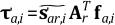
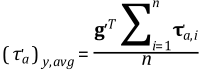
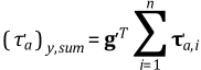
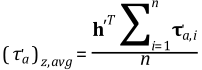
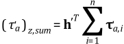
The contact force at the i^th contact point acting on the action side and the torque generated by the i^th contact force, each measured in the reference frame, are calculated as follows.

(8–7)

(8–8)

(8–9)

Where is the contact force acting on the action body at the i^th contact point, is the position of the i^th contact point, is the position of the reference marker, and is the orientation matrix of the reference marker. For more information, see Intermittent Contact Force.

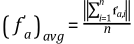
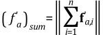
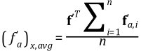
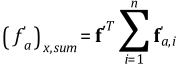
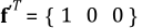
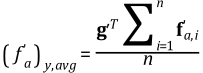
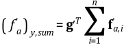
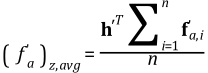
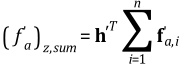
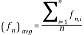
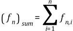
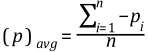
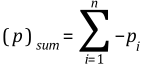
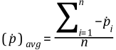
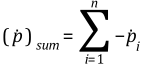
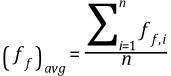
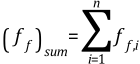
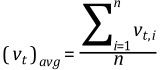
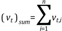
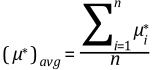
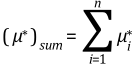
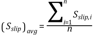
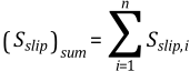
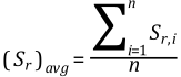
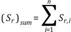
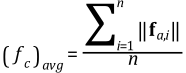
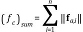
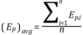
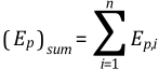
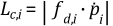
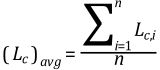
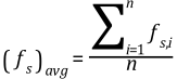
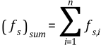
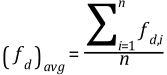
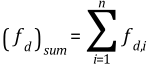
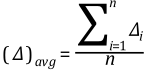
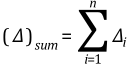
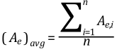
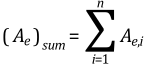
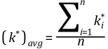
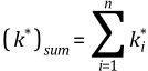
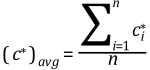
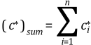
Contact functions support result types that return the average, sum, minimum, or maximum value at each contact point. Depending on the result type, predefined constant values AVG_RES, SUM_RES, MIN_RES, and MAX_RES or corresponding integer values can be entered. The return according to each result type is as follows.

Figure 8.10: Supported contact functions for each contact type

Result Type	Predefined Constant	Description	Return Value
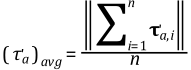
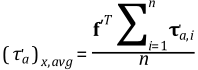
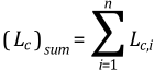
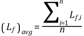
Average	AVG_RES(0)	Returns the average of the values at each contact point.
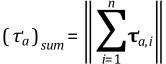
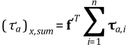
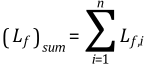
Sum	SUM_RES(1)	Returns the sum of the values at each contact point.
Min	MIN_RES(2)	Returns the minimum value among the values at each contact point.
Max	MAX_RES(3)	Returns the maximum value among the values at each contact point.

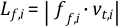
Where n is the number of contact points and is real value at the i^th contact point.

Note that average and summed contact forces or torques acting on the target (action) side are calculated from vector sums. For minimum and maximum, these are a comparison of the magnitudes of the vectors at each contact point.

Contact Functions can be defined as shown in the table below. If the reference marker is not defined, contact functions that measure force and torque will be automatically set to the inertia reference marker. The position and orientation of the inertia reference marker are the zero vector and the identity matrix, respectively. Zero is returned if there are no points in contact.

Figure 8.11: Contact Functions

Functions

Description

CONTFSUM(E1,E2)

Definition

The magnitude of the contact force on the target (action) side.

Input (E1,E2)

E1: argument ID of the contact

E2: result type (one of AVG_RES, SUM_RES, MIN_RES, or MAX_RES)

Return Value

Result Type	Return Value
Average
Sum
Min
Max

Where n is the number of contact points and Contact Functions is i^th contact force on the target (action) side which is defined in Equation 8–7

Example

CONTFSUM(p1,AVG_RES)

CONTFX(E1,E2,{E3})

Definition

The x-component of the contact force on the target (action) side with respect to the reference marker.

Input (E1,E2,E3)

E1: argument ID of the contact

E2: result type (one of AVG_RES, SUM_RES, MIN_RES, or MAX_RES)

E3: argument ID of the reference marker

Return Value

Result Type	Return Value
Average
Sum
Min
Max

Where Contact Functions , n is the number of contact points and is i^th contact force on the target (action) side with respect to the reference frame which is defined in Equation 8–7.

Example

CONTFX(p1,AVG_RES), CONTFX(p1,SUM_RES,p2)

CONTFY(E1,E2,{E3})

Definition

The y-component of the contact force on the target (action) side with respect to the reference marker.

Input (E1,E2,E3)

E1: argument ID of the contact

E2: result type (one of AVG_RES, SUM_RES, MIN_RES, or MAX_RES)

E3: argument ID of the reference marker

Return Value

Result Type	Return Value
Average
Sum
Min
Max

Where Contact Functions , n is the number of contact points and is i^th contact force on the target (action) side with respect to the reference frame which is defined in Equation 8–7.

Example

CONTFY(p1,AVG_RES), CONTFY(p1,SUM_RES,p2)

CONTFZ(E1,E2,{E3})

Definition

The z-component of the contact force on the target (action) side with respect to the reference marker.

Input (E1,E2,E3)

E1: argument ID of the contact

E2: result type (one of AVG_RES, SUM_RES, MIN_RES, or MAX_RES)

E3: argument ID of the reference marker

Return Value

Result Type	Return Value
Average
Sum
Min
Max

where Contact Functions , n is the number of contact points and is i^th contact force on the target (action) side with respect to the reference frame which is defined in Equation 8–7.

Example

CONTFZ(p1,AVG_RES), CONTFZ(p1,SUM_RES,p2)

CONTTSUM(E1,E2,{E3})

Definition

The magnitude of the torque due to the contact force on the target (action) side with respect to the reference marker.

Input (E1,E2,E3)

E1: argument ID of the contact

E2: result type (one of AVG_RES, SUM_RES, MIN_RES, or MAX_RES)

E3: argument ID of the reference marker

Return Value

Result Type	Return Value
Average
Sum
Min
Max

Where n is the number of contact points and Contact Functions is the torque generated by the i^th contact force on the target (action) side with respect to the reference frame which is defined in Equation 8–8.

Example

CONTTSUM(p1,AVG_RES), CONTTSUM(p1,SUM_RES,p2)

CONTTX(E1,E2,{E3})

Definition

The x-component of the torque due to the contact force on the target (action) side with respect to the reference marker.

Input (E1,E2,E3)

E1: argument ID of the contact

E2: result type (one of AVG_RES, SUM_RES, MIN_RES, or MAX_RES)

E3: argument ID of the reference marker

Return Value

Result Type	Return Value
Average
Sum
Min
Max

Where Contact Functions , n is the number of contact points and is the torque generated by the i^th contact force on the target (action) side with respect to the reference frame which is defined in Equation 8–8.

Example

CONTTX(p1,AVG_RES), CONTTX(p1,SUM_RES,p2)

CONTTY(E1,E2,{E3})

Definition

The y-component of the torque due to the contact force on the target (action) side with respect to the reference marker.

Input (E1,E2,E3)

E1: argument ID of the contact

E2: result type (one of AVG_RES, SUM_RES, MIN_RES, or MAX_RES)

E3: argument ID of the reference marker

Return Value

Result Type	Return Value
Average
Sum
Min
Max

Example

CONTTY(p1,AVG_RES), CONTTY(p1,SUM_RES,p2)

CONTTZ(E1,E2,{E3})

Definition

The z-component of the torque due to the contact force on the target (action) side with respect to the reference marker.

Input (E1,E2,E3)

E1: argument ID of the contact

E2: result type (one of AVG_RES, SUM_RES, MIN_RES, or MAX_RES)

E3: argument ID of the reference marker

Return Value

Result Type	Return Value
Average
Sum
Min
Max

Example

CONTTZ(p1,AVG_RES), CONTTZ(p1,SUM_RES,p2)

CONTNF(E1,E2)

Definition

The contact normal force on the target (action) side at the contact points.

Input (E1,E2)

E1: argument ID of the contact

E2: result type (one of AVG_RES, SUM_RES, MIN_RES, or MAX_RES)

Return Value

Result Type	Return Value
Average
Sum
Min
Max

Where n is the number of contact points and Contact Functions is the normal force at the i^th contact point which is defined in Equation 6–49.

Example

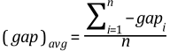
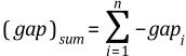
CONTGAP(E1,E21)

Definition

The contact gap at the contact points.

Input (E1,E2)

E1: argument ID of the contact

E2: result type (one of AVG_RES, SUM_RES, MIN_RES, or MAX_RES)

Return Value

Result Type	Return Value
Average
Sum
Min
Max

Where n is the number of contact points and Contact Functions is the contact gap at the i^th contact point which is defined in Equation 6–21.

Note: According to Equation 6–21, the contact gap is calculated as positive by the solver, and a positive contact gap is reported with a negative sign to aid user comprehension.

Example

CONTGAP(p1,AVG_RES)

CONTPENE(E1,E2)

Definition

The contact penetration at the contact points.

Input (E1,E2)

E1: argument ID of the contact

E2: result type (one of AVG_RES, SUM_RES, MIN_RES, or MAX_RES)

Return Value

Result Type	Return Value
Average
Sum
Min
Max

Where n is the number of contact points and Contact Functions is the contact penetration at the i^th contact point which is defined in Equation 6–19.

Note: According to Equation 6–19, contact penetration is calculated as negative by the solver, and negative contact penetration is reported with a positive sign to aid user comprehension.

Example

CONTPENE(p1,AVG_RES)

CONTDPENE(E1,E2)

Definition

The contact penetration velocity at the contact points.

Input (E1,E2)

E1: argument ID of the contact

E2: result type (one of AVG_RES, SUM_RES, MIN_RES, or MAX_RES)

Return Value

Result Type	Return Value
Average
Sum
Min
Max

Where n is the number of contact points and Contact Functions is the contact penetration velocity at the i^th contact point which is defined in Equation 6–54.

Note: According to Equation 6–54, contact penetration velocity that increases contact penetration is calculated as negative by the solver. In order to aid user comprehension and indicate penetration velocity that increases contact penetration with a positive sign, negative penetration velocity is reported.

Example

CONTDPENE(p1,AVG_RES)

CONTFF(E1,E2)

Definition

The contact friction force at the contact points.

Input (E1,E2)

E1: argument ID of the contact

E2: result type (One of AVG_RES, SUM_RES, MIN_RES, or MAX_RES)

Return Value

Result Type	Return Value
Average
Sum
Min
Max

Where n is the number of contact points and Contact Functions is the contact friction force at the i^th contact point which is defined in Equation 6–69.

Example

CONTFF(p1,AVG_RES)

CONTTVEL(E1,E2)

Definition

The tangential velocity, which is the relative velocity in the tangential direction at the contact points.

Input (E1,E2)

E1: argument ID of the contact

E2: result type (One of AVG_RES, SUM_RES, MIN_RES, or MAX_RES)

Return Value

Result Type	Return Value
Average
Sum
Min
Max

Where n is the number of contact points and Contact Functions is the tangential velocity at the i^th contact point.

Example

CONTTVEL(p1,AVG_RES)

CONTFCOEFF(E1,E2)

Definition

The friction coefficient at the contact points.

Input (E1,E2)

E1: argument ID of the contact

E2: result type (One of AVG_RES, SUM_RES, MIN_RES, or MAX_RES)

Return Value

Result Type	Return Value
Average
Sum
Min
Max

Where n is the number of contact points and Contact Functions is the contact friction force at the i^th contact point which is defined in Equation 6–69.

Example

CONTFCOEFF(p1,AVG_RES)

CONTSTAT(E1,E2)

Definition

The contact slip status at the contact points.

0 : No Contact
1 : Stiction
2 : Static ( Deformation > Max Stiction Deformation and Tangent Velocity < Stiction Velocity)
3 : Transient (Stiction Velocity < Tangent Velocity < Dynamic Threshold)
4 : Dynamic (Dynamic Threshold < Tangent Velocity)

Input (E1,E2)

E1: argument ID of the contact

E2: result type (One of AVG_RES, SUM_RES, MIN_RES, or MAX_RES)

Return Value

Result Type	Return Value
Average
Sum
Min
Max

Where n is the number of contact points and Contact Functions is the slip status at the i^th contact point.

Example

CONTSTAT(p1,AVG_RES)

CONTSLIPRA(E1,E2)

Definition

The slip ratio at the contact points.

Input (E1,E2)

E1: argument ID of the contact

E2: result type (One of AVG_RES, SUM_RES, MIN_RES, or MAX_RES)

Return Value

The slip ratio at the i^th contact point Contact Functions is calculated as follows:

Contact Functions

where the variables Contact Functions and are the target (action) and contact (base) tangential velocity at the contact point.

Result Type	Return Value
Average
Sum
Min
Max

where n is the number of contact points.

Example

CONTSLIPRA(p1,AVG_RES)

CONTPFMAG(E1,E2)

Definition

The force magnitude at the contact points.

Input (E1,E2)

E1: argument ID of the contact

E2: result type (One of AVG_RES, SUM_RES, MIN_RES, or MAX_RES)

Return Value

Result Type	Return Value
Average
Sum
Min
Max

Where n is the number of contact points and Contact Functions is the slip status at the i^th contact point.

Example

CONTPFMAG(p1,AVG_RES)

CONTPOENER(E1,E2)

Definition

The contact potential energy due to the contact spring force at the contact points.

Input (E1,E2)

E1: argument ID of the contact

E2: result type (One of AVG_RES, SUM_RES, MIN_RES, or MAX_RES)

Return Value

The potential energy at the i^th contact point Contact Functions is calculated as follows:

Contact Functions

where Contact Functions is the exponent of penetration in Equation 6–52, is the contact spring force and is the contact penetration at the i^th contact point.

Result Type	Return Value
Average
Sum
Min
Max

Where n is the number of contact points.

Example

CONTPOENER(p1,AVG_RES)

CONTNLOSS(E1,E2)

Definition

The loss by the contact damping at the contact points.

Input (E1,E2)

E1: argument ID of the contact

E2: result type (One of AVG_RES, SUM_RES, MIN_RES, or MAX_RES)

Return Value

The loss by contact damping at the i^th contact point Contact Functions is calculated as follows:

Contact Functions

where Contact Functions is the contact spring force and is the contact penetration at the i^th contact point.

Result Type	Return Value
Average
Sum
Min
Max

Where n is the number of contact points.

Example

CONTNLOSS(p1,AVG_RES)

CONTFLOSS(E1,E2)

Definition

The loss by contact friction at the contact points.

Input (E1,E2)

E1: argument ID of the contact

E2: result type (One of AVG_RES, SUM_RES, MIN_RES, or MAX_RES)

Return Value

The loss by contact friction at the i^th contact point Contact Functions is calculated as follows:

Contact Functions

where Contact Functions is the contact spring force and is the contact penetration at the i^th contact point.

Result Type	Return Value
Average
Sum
Min
Max

Where n is the number of contact points.

Example

CONTFLOSS(p1,AVG_RES)

CONTKF(E1,E2)

Definition

The contact spring force at the contact points.

Input (E1,E2)

E1: argument ID of the contact

E2: result type (One of AVG_RES, SUM_RES, MIN_RES, or MAX_RES)

Return Value

Result Type	Return Value
Average
Sum
Min
Max

Where n is the number of contact points and Contact Functions is the contact spring force at the i^th contact point. See Intermittent Contact Force for more information.

Example

CONTKF(p1,AVG_RES)

CONTCF(E1,E2)

Definition

The contact damping force at the contact points.

Input (E1,E2)

E1: argument ID of the contact

E2: result type (One of AVG_RES, SUM_RES, MIN_RES, or MAX_RES)

Return Value

Result Type	Return Value
Average
Sum
Min
Max

Where n is the number of contact points and Contact Functions is the contact damping force at the i^th contact point. See Intermittent Contact Force for more information.

Example

CONTCF(p1,AVG_RES)

CONTCREEP(E1,E2)

Definition

The creep at the contact points.

Input (E1,E2)

E1: argument ID of the contact

E2: result type (One of AVG_RES, SUM_RES, MIN_RES, or MAX_RES)

Return Value

Result Type	Return Value
Average
Sum
Min
Max

Where n is the number of contact points and Contact Functions is the creep distance at the i^th contact point. See Friction in a Translational Joint for more information.

Example

CONTCREEP(p1,AVG_RES)

CONTAREA(E1,E2)

Definition

The contact area at contact points.

Input (E1,E2)

E1: argument ID of the contact

E2: result type (One of AVG_RES, SUM_RES, MIN_RES, or MAX_RES)

Return Value

Result Type	Return Value
Average
Sum
Min
Max

Where n is the number of contact points and Contact Functions is the contact damping force at the i^th contact point as defined in Equation 6–60.

This function returns 0 if the Node Only option is disabled. When the Point Check option is set to Action & Base Points or Program Controlled, the contact area is calculated based on target (action) points. In other cases, the contact area is calculated based on the target (action) or contact (base) points set in Point Check. See General Contact Output for more information.

Example

CONTAREA(p1,AVG_RES)

CONTKCOEFF(E1,E2)

Definition

The contact stiffness coefficient at the contact points.

Input (E1,E2)

E1: argument ID of the contact

E2: result type (One of AVG_RES, SUM_RES, MIN_RES, or MAX_RES)

Return Value

Result Type	Return Value
Average
Sum
Min
Max

Where n is the number of contact points and Contact Functions is the contact stiffness coefficient at the i^th contact point as defined in Equation 6–52 and Equation 6–61.

Example

CONTKCOEFF(p1,AVG_RES)

CONTCCOEFF(E1,E2)

Definition

The contact damping coefficient at the contact points.

Input (E1,E2)

E1: argument ID of the contact

E2: result type (One of AVG_RES, SUM_RES, MIN_RES, or MAX_RES)

Return Value

Result Type	Return Value
Average
Sum
Min
Max

Where n is the number of contact points and Contact Functions is the contact damping coefficient at the i^th contact point. See Figure 6.63: Damping coefficient of contact force and Figure 6.69: Damping coefficient(ratio) of contact force in Intermittent Contact Force for more information.

Example

CONTCCOEFF(p1,AVG_RES)

CONTNPOINT(E1)

Definition

The number of contact points.

Input (E1)

E1: argument ID of the contact

Return Value

The number of contact points Contact Functions

Example

CONTNPOINT(p1)

8.1.9. System Element Functions

System Element Functions are used to measure variables generated from equation entities. The name or argument ID of the equation entity is needed to define the function. The returned value is a variable which may be defined as follows.

(8–10)

(8–11)

(8–12)

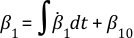
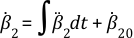
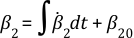
where E, D₁ and D₂ are the variable equation and first and second order differential equations, respectively. The parameters of the equations refer to position, velocity, acceleration, variables, force, torque and time. For the first and second order differential equations, the time integrated values can be calculated from the following equations.

(8–13)

(8–14)

(8–15)

where , and are the initial conditions of the differential equations.

System Element Functions can be defined as shown in the table below.

Figure 8.12: System Element Functions

Functions	Description
VARVAL(E1)	Definition	The value of the variable equation.
	Input (E1)	E1 is the name or argument ID of the variable equation.
	Return Value	The value of Equation 8–10 will be returned.
	Example	VARVAL(p1)
DIF10(E1)	Definition	The integrated variable of the 1st order differential equation.
	Input (E1)	E1 is the name or argument ID of the 1st order differential equation.
	Return Value	The value of Equation 8–13 will be returned.
	Example	DIF10(p1)
DIF11(E1)	Definition	The differential variable of the 1st order differential equation.
	Input (E1)	E1 is the name or argument ID of the 1st order differential equation.
	Return Value	The value of Equation 8–11 will be returned.
	Example	DIF11(p1)
DIF20(E1)	Definition	The double integrated variable of the 2nd order differential equation.
	Input (E1)	E1 is the name or argument ID of the 2nd order differential equation.
	Return Value	The value of Equation 8–15 will be returned.
	Example	DIF20(p1)
DIF21(E1)	Definition	The integrated variable of the 2nd order differential equation.
	Input (E1)	E1 is the name or argument ID of the 2nd order differential equation.
	Return Value	The value of Equation 8–14 will be returned.
	Example	DIF21(p1)
DIF22(E1)	Definition	The differential variable of the 2nd order differential equation.
	Input (E1)	E1 is the name or argument ID of the 2nd order differential equation.
	Return Value	The value of Equation 8–12 will be returned.
	Example	DIF22(p1)

8.1.10. Arithmetic IF Functions

An Arithmetic IF function represents a conditional function and can be defined as shown in the table below.

Figure 8.13: Arithmetic IF Functions

Functions	Description
IF(E1,E2,E3,E4)	Definition	The conditional function.
	Input (E1,E2,E3,E4)	E1, E2, E3 and E4 can be defined as constant values, variables or formulas.
	Return Value	A value will be returned oaacrding to the following conditions. 1) E1 < 0 : E2 2) E1 = 0 : E3 3) E1 > 0 : E4
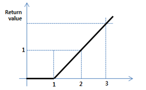
	Example	IF(time-1,0,0,time-1) The values for time are returned as shown in the figure below.

Figure 8.14: Example of an IF Function

8.1.11. Interpolation Functions

These functions return the interpolated value for the given independent variable with the specified Spline and can be defined as shown in the Interpolation Functions table below.

(8–16)

where the independent variable x must be between the minimum and maximum values of the spline. If the variable is outside this range, the function will return the extrapolated value with the last slope of the spline. The number of values in the data set of the spline must be greater than three. For the Akima interpolation method, the interpolation function of Equation 8–16 can be expressed as follows.

(8–17)

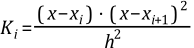
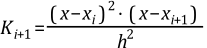
where the coefficients are defined as follows.

(8–18)

(8–19)

(8–20)

(8–21)

(8–22)

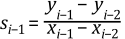
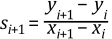
The independent variable x is a value between x_i and x_i+1, which are defined in the spline. y_i and y_i+1 are corresponding values for x_i and x_i+1. In Equation 8–17, the slopes of y′ are defined by the following equations.

(8–23)

(8–24)

(8–25)

(8–26)

(8–27)

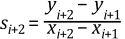(8–28)

For the linear interpolation method, the interpolation function of Equation 8–16 can be expressed as follows.

(8–29)

where the slope of s_i+1 is defined in Equation 8–27.

For the three-dimension interpolation method, assume that the function z(x,y) in a rectangle bounded by four straight lines x=x₁, x=x₂, y=y₁ and y=y₂ can be expressed by a bicubic polynomial in x and y, and that the polynomial is determined by the values of the function z and its partial derivatives z_x, z_y and z_xy at four corner points (x₁, y₁), (x₁, y₂), (x₂, y₁) and (x₂, y₂).

The interpolation function can be expressed as follows.

(8–30)

where the p coefficients are

(8–31)

(8–32)

(8–33)

(8–34)

(8–35)

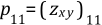(8–36)

(8–37)

(8–38)

(8–39)

(8–40)

(8–41)

(8–42)

(8–43)

(8–44)

(8–45)

(8–46)

and where

(8–47)

(8–48)

(8–49)

(8–50)

and where

(8–51)

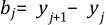(8–52)

(8–53)

(8–54)

(8–55)

For more details, see the reference below.

Hiroshi Akima, A Method of Bivariate Interpolation and Smooth Surface Fitting Based on Local Procedures, Communications of the ACM, Jan, 1974

Figure 8.15: Interpolation Functions

Functions	Description
AKISPL (E1,E2,E3,E4)	Definition	Use to get an interpolated function value for the independent variable with the Akima interpolation method in Equation 8–17. For 2D Splines, the interpolation is performed to determine the y value based on the given x value. In the case of 3D Splines, the interpolation is conducted to ascertain the y value, taking into account both the x and z values.
	Input (E1,E2,E3,E4)	E1 is the independent variable x and must be a real number or an expression. E2, for 3D splines, represents the independent variable z and must be a real number or an expression. For 2D splines, E2 must be zero due to the absence of a z-dimension. E3 is the name of the argument associated with the targeted spline. E4 determines the order of the returned value. For 3D splines, only order `0` is supported.
	Return Value	A value will be returned according to the order (E4) as follows. 0 → 1 → 2 → Orders `1` and `2` are only supported for 2D splines.
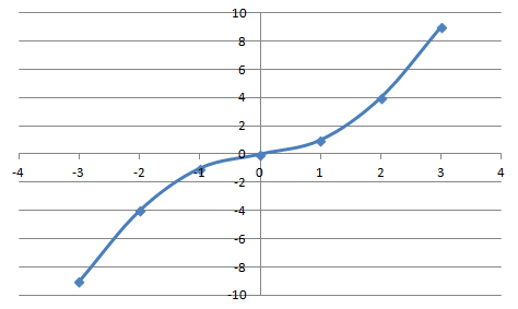
	Example for 2D Splines	AKISPL(time,0,p1,0) When the spline is defined as shown in Figure 8.16: Example of a 2D Spline, the values for time will be returned as shown in the figure below.
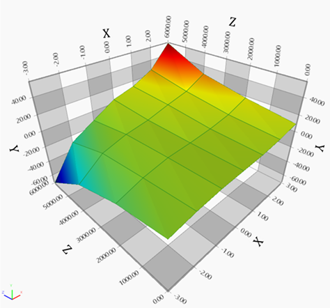
	Example for 3D Splines	AKISPL(time,WZ(p2,p2,p3),p1,0) In this example, p2 and p3 are the names of the arguments corresponding to the action and base markers of a revolute joint, respectively. When the spline is defined as shown in Figure 8.17: Example of a 3D Spline, the values for time will be returned as shown in the figure below.
LININT (E1,E2,E3,E4)	Definition	Use to get an interpolated function value for the independent variable using the linear interpolation method in Equation 8–29.
	Input (E1,E2,E3,E4)	E1 is real or expression type and the independent variable x. E2 is integer type and must be zero. E3 is the name or argument ID of the spline. E4 is the order of the returned value.
	Return Value	A value will be returned under the condition of the order (E4) as follows. 1) 0 → 2) 1 → 3) 2 →
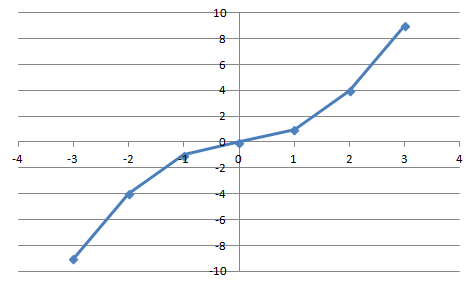
	Example	LININT(time,0,p1,0) When the spline is defined as shown in the Figure 8.16: Example of a 2D Spline table below, the values for time will be returned as shown in the figure below.

Figure 8.16: Example of a 2D Spline

X	Y
-3	-9
-2	-4
-1	-1
0	0
1	1
2	4
3	9

Figure 8.17: Example of a 3D Spline

	Z Data
X Data		0	2000	4000	6000
	-3	-9	-18	-36	-72
	-2	-4	-8	-13	-29
	-1	-1	-2	-4	-12
	0	0	0	1	5
	1	1	3	9	13
	2	4	8	16	27
	3	9	19	30	56

Figure 8.17: Example of a 3D Spline shows Y Data as values determined by corresponding X Data and Z Data, with X Data along the vertical axis, Z Data along the horizontal axis, and Y Data at their intersections.

Note: The input data for splines must follow these rules.

For x-axis and z-axis data:

The data must be entered in order from smallest to largest.
There must be no duplicate values.
There must be no empty data.
There must be at least 4 data points.

For y-axis data:

There must be no empty data.

8.1.12. Predefined Functions

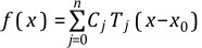
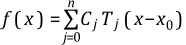
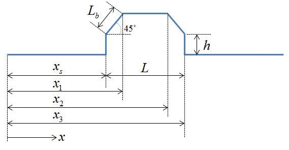
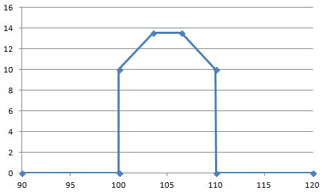
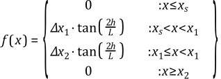
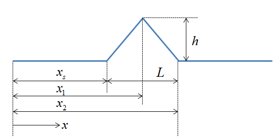
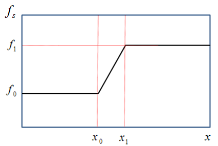
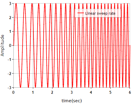
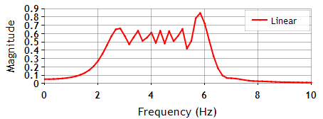
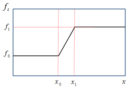
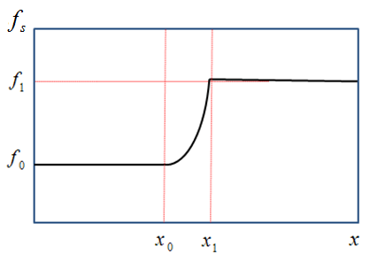
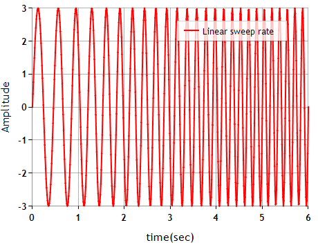
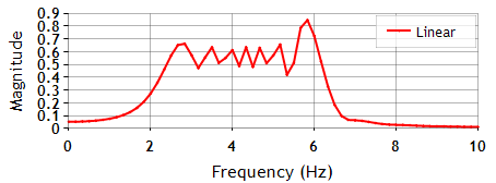
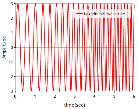
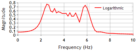
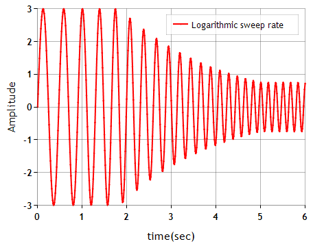
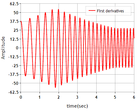
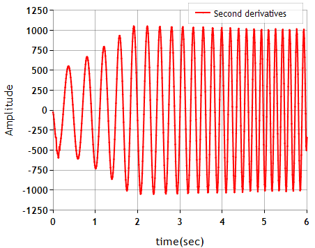
These functions will help to build a mechanical system and can be defined as shown in the table below.

Figure 8.18: Predefined Functions

Functions	Description
CHEBY (E1,E2,E3,…,EN)	Definition	Use to define the Chebyshev polynomial as in the following equations. where the functions of T_j are recursively defined as follows.
	Input (E1,E2, E3,… ,EN)	E1 is the independent variable x (real or expression type).
		E2 is the offset x₀ (real or expression type).
		E3 is the first polynomial coefficient C₀ (real or expression type).
		EN is the last polynomial coefficient C_n (real or expression type). The number of polynomial is less than or equal to 31.
	Return Value	A return value is f(x).
	Example	CHEBY (time,0.0,1.0,1.0,2.0)
POLY (E1,E2,E3,…,EN)	Definition	Use to define the standard polynomial as in the following equation. where the function T_j is defined as follows.
	Input (E1,E2, E3,… ,EN)	E1 is the independent variable x (real or expression type).
		E2 is the offset x₀ (real or expression type).
		E3 is the first polynomial coefficient C₀ (real or expression type).
		EN is the last polynomial coefficient C_n (real or expression type). The number of polynomials is less than or equal to 31.
	Return Value	A return value is f(x).
	Example	POLY (time,0.0,1.0,1.0,2.0)
HAVSIN(E1,E2,E3,E4,E5)	Definition	Use to define the Haversine as in the following equations. where
	Input (E1,E2, E3,E4 ,E5)	E1 is the independent variable x (real or expression type).
		E2 is the value x₀ at which the function starts (real or expression type).
		E3 is the initial value h₀ (real or expression type).
		E4 is the value x₁ at which the function ends (real or expression type).
		E5 is the final value h₁ (real or expression type).
	Return Value	A return value is f(x).
	Example	HAVSIN (time,1.0,-10.0,2.0,10.0)
STEP(E1,E2,E3,E4,E5)	Definition	Use to define the approximated Heaviside step function with cubic polynomial as in the following equations. where
	Input (E1,E2, E3,E4 ,E5)	E1 is the independent variable x (real or expression type).
		E2 is the value x₀ at which the function starts (real or expression type).
		E3 is the initial value h₀ (real or expression type).
		E4 is the value x₁ at which the function ends (real or expression type).
		E5 is the final value h₁ (real or expression type).
	Return Value	The return value is f(x).
	Example	STEP (time,0.9,100.0,2.0,-100.0)
FORCOS (E1,E2,E3,E4,…,EN)	Definition	Use to define the fourier cosine series as following equations. where the function T_j is defined as follows.
	Input (E1,E2, E3,E4,…, EN)	E1 is the independent variable x (real or expression type).
		E2 is the offset x₀ (real or expression type).
		E3 is the frequency w (real or expression type).
		E4 is the first amplitude C₀ (real or expression type).
		EN is the last amplitude C_n (real or expression type). The number of series is less than or equal to 31.
	Return Value	The return value is f(x).
	Example	FORCOS(time,0.0,10.0,1.0,1.0,2.0)
FORSIN (E1,E2,E3,E4,…,EN)	Definition	Use to define the fourier sine series as following equations. where the function T_j is defined as follows.
	Input (E1,E2, E3,E4,…, EN)	E1 is the independent variable x (real or expression type).
		E2 is the offset x₀ (real or expression type).
		E3 is the frequency w (real or expression type).
		E4 is the first amplitude C₀ (real or expression type).
		EN is the last amplitude C_n (real or expression type). The number of series is less than or equal to 31.
	Return Value	The return value is f(x).
	Example	FORSIN(time,0.0,10.0,1.0,1.0,2.0)
SHF (E1,E2,E3,E4,E5,E6)	Definition	Use to define the simple harmonic function as following equations.
	Input (E1,E2, E3,E4,E5, E6)	E1 is the independent variable x (real or expression type).
		E2 is the offset x₀ (real or expression type).
		E3 is the amplitude A (real or expression type).
		E4 is the frequency w (real or expression type).
		E5 is the phase angle ϕ (real or expression type).
		E6 is the mean value of y₀ (real or expression type).
	Return Value	The return value is f(x).
	Example	SHF(time,0.0,10.0,100.0,0.0,50.0)
IMPACT (E1,E2,E3,E4,E5, E6,E7)	Definition	Use to define the impact function as following equations. When the independent variable is a function of distance, this function can represent a simple contact force as shown in the figure showing the IMPACT function below. where IMPACT function
	Input (E1,E2, E3,E4,E5, E6,E7)	E1 is the independent variable x (real or expression type). This variable may be a displacement function.
		E2 is the time derivative of x (real or expression type).
		E3 is the radius R (real type). When the independent variable x is less than this value, the force is will be generated.
		E4 is the contact stiffness k (non-negative real type).
		E5 is the contact exponent e (positive real type).
		E6 is the maximum damping coefficient c_max (non-negative real type).
		E7 is the boundary penetration d (positive real type).
	Return Value	The return value is .
	Example	IMPACT(DY(p1,p2),VY(p1,p2),10.0,1000.0,1.0,1.0,1.0) When VY is zero, IMPACT will return for the displacement as shown in the figure below.
BISTOP (E1,E2,E3,E4,E5, E6,E7,E8)	Definition	Use to define the bi-stop function as in the following equations. When the independent variable is a function of distance, this function can represent a gap contact as shown in the BISTOP function figure below. where BISTOP function
	Input (E1,E2, E3,E4,E5, E6,E7,E8)	E1 is the independent variable x (real or expression type). This variable may be a displacement function.
		E2 is the time derivative of x (real or expression type).
		E3 is the radius x₁ (real type). When the independent variable x is less than this value, the force is will be generated.
		E4 is the radius x₂ (real type). When the independent variable x is greater than this value, the force is will be generated.
		E5 is the contact stiffness k (non-negative real type).
		E6 is the contact exponent e (positive real type).
		E7 is the maximum damping coefficient c_max (non-negative real type).
		E8 is the boundary penetration d (positive real type).
	Return Value	The return value is .
	Example	BISTOP (DY(p1,p2),VY(p1,p2),20.0,21.0,1000.0,1.0,1.0,1.0) When VY is zero, the bi-stop will return for the displacement as shown in the following figure.
PLANK (E1,E2,E3,E4,E5)	Definition	Use to define the Plank function as in the following equations. When the independent variable is a function of distance, this function can represent a bump in a road as shown in the PLANK function figure below. PLANK function
	Input (E1,E2, E3,E4,E5)	E1 is the independent variable x (real or expression type). This variable may be a displacement function.
		E2 is the starting length x_s (real type). When the independent variable of x is less than this value, the function is will return zero.
		E3 is the bump length L (real type).
		E4 is the beveled length L_b (real type).
		E5 is the bump height h (real type).
	Return Value	The return value is f(x).
	Example	PLANK (DX(p1,p2),100.0,10.0,5.0,10.0)
ROOF (E1,E2,E3,E4)	Definition	Use to define the roof function as in the following equations. When the independent variable is a function of distance, this function can represent a bump in a road as shown in the ROOF function figure below. ROOF function
	Input (E1,E2, E3,E4)	E1 is the independent variable x (real or epxression type). This variable may be a displacement function.
		E2 is the starting length x_s (real type). When the independent variable of x is less than this value, the function is will return zero.
		E3 is the bump length L.
		E4 is the bump height h.
	Return Value	The return value is f(x).
	Example	ROOF (DX(p1,p2),100.0,10.0 ,10.0)
STEP0 (E1,E2,E3,E4)	Definition	Use to define the step function without a transition as shown in the STEP0 figure figure below and in the following equations. SETP0 function
	Input (E1,E2, E3,E4)	E1 is the independent variable x (real or expression type).
		E2 is the starting length x_s (real type). When the independent variable x is less than this value, the function is will return zero.
		E3 is the length L (real type).
		E4 is the height h (real type).
	Return Value	The return value is f(x).
	Example	STEP0 (DX(p1,p2),100.0,10.0 ,10.0)
SWEEP (E1,E2,E3,E4,E5, E6, E7)	Definition	Use to define the sweep function which generates a sine wave in the range of specified start and end frequencies with linear sweep rate as in the following equations. where the spectral frequency of the linear sweep rate can be defined as shown in the figure below. Spectral frequency with linear sweep rate
	Input (E1,E2, E3,E4,E5, E6,E7)	E1 is the independent variable x (real or expression type). This value must be greater than or equal to zero. In general, the variable may be defined as a time.
		E2 is the amplitude A (real type).
		E3 is the starting variable x₀ (real type). This value must be greater than or equal to zero.
		E4 is the starting frequency f₀ (real type). This value must be greater than zero.
		E5 is the ending variable x₁ (real type). This value must be greater than the starting variable.
		E6 is the ending frequency f₁ (real type). This value must be greater than zero.
		E7 is the step size Δt (real type) which is not used in Motion solver.
	Return Value	The return value is y(x).
	Example	SWEEP (time, 3.0, 0.0, 2.0, 5.0, 6.0, 0.01) This function will return values for the time as follows. The results above will be shown in the frequency domain as follows.
SINE_SWEEP (E1,E2,E3,E4,E5, E6, E7,E8)	Definition	Use to define the advanced sweep function which generates a sine wave in the range of specified start and end frequencies with linear and logarithm sweep rate as in the following equations. where the spectral frequencies of linear and logarithm sweep rate can be defined as shown in the figures below. Spectral frequency with linear sweep rate Spectral frequency with logarithm sweep rate
	Input (E1,E2, E3,E4,E5, E6,E7,E8)	E1 is the independent variable x (real or expression type). This value must be greater than or equal to zero. In general, the variable may be defined as a time.
		E2 is the amplitude A (real type).
		E3 is the starting variable x₀ (real type). This value must be greater than or equal to zero.
		E4 is the starting frequency f₀ (real type). This value must be greater than zero.
		E5 is the ending variable x₁ (real type). This value must be greater than the starting variable.
		E6 is the ending frequency f₁ (real type). This value must be greater than zero.
		E7 is the cut-off frequency f_c (real type). This value must be greater than zero.
		E8 is integer type and the sweep rate type. When this is 1, the linear sweep rate is used in the function. When this is 2, the logarithm sweep rate is used in the function.
	Return Value	The return value is y(x).
	Example	1. SINE_SWEEP (time, 3.0, 0.0, 2.0, 5.0, 6.0, 10.0,1) This function will return values for the time as follows. The results above will be shown in the frequency domain as follows. 2. SINE_SWEEP (time, 3.0, 0.0, 2.0, 5.0, 6.0, 10.0,2) This function will return values for the time as follows. The results above will be shown in the frequency domain as follows. 3. SINE_SWEEP (time, 3.0, 0.0, 2.0, 5.0, 6.0, 3.0,2) This function will return values for the time as follows. The first derivatives of the function will be as follows. The second derivatives of the function will be as follows.

8.1.13. Interface Parameters and Sub-Entity Functions

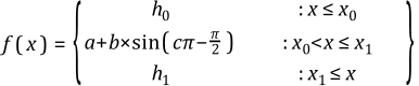
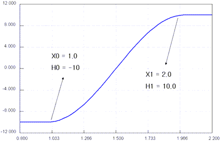
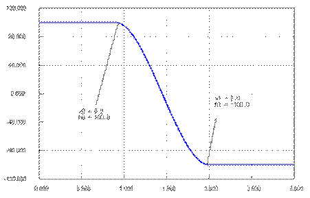
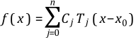
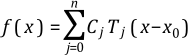
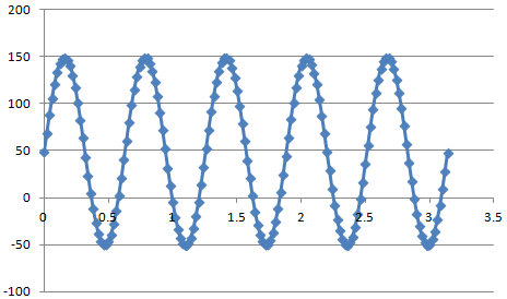
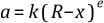
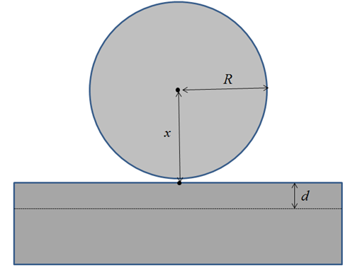
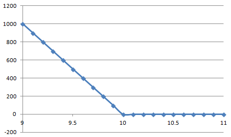
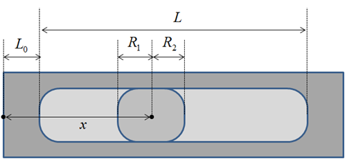
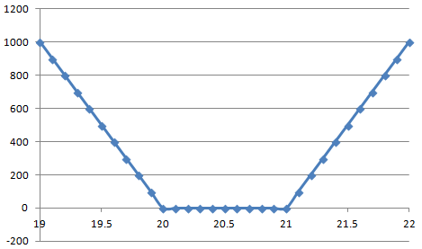
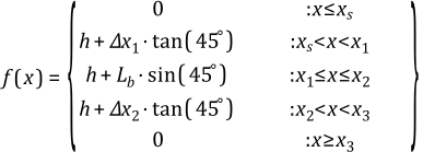
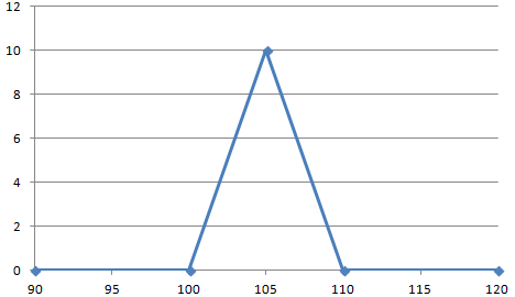
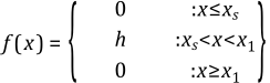
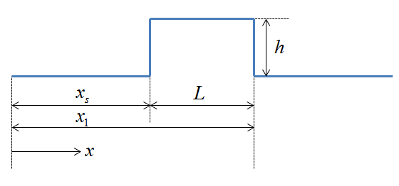
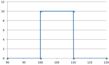
These functions return the value of interface variables under the co-simulation or user-defined array and can be defined as shown in the table below.

Figure 8.19: Interface Parameters and Sub-Entity Functions

Functions	Description
SINPUT(E1)	Definition	The variable of S-Input.
	Input (E1)	E1 is the name or argument ID of the SINPUT.
	Return Value	A variable value of the specified SINPUT will be returned.
	Example	SINPUT(p1)
SOUTPUT(E1)	Definition	The variable of S-Output.
	Input (E1)	E1 is the name or argument ID of the SOUTPUT.
	Return Value	A variable value of the specified SOUTPUT will be returned.
	Example	SOUTPUT (p1)
ARRAY(E1,E2)	Definition	The variable of Arrays.
	Input (E1)	E1 is the name or argument ID of the ARRAY.
	Input (E2)	E2 is the sequence of a value which is contained in the array. If you want to get the first value of the array, E2 must be set to zero.
	Return Value	A variable value of the specified ARRAY will be returned.
	Example	ARRAY (p1,3) The 4^th value of the array `p1` will be returned.

8.1.14. User Defined Python Functions

Function expressions can make use of functions contained in imported python code. See User Defined Python Code for more information.

8.1.15. Function Expression Output

The return value of a Function Expression is reported in the Motion Postprocessor.