


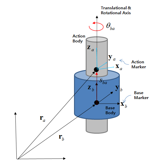
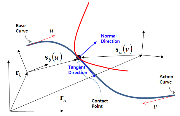
Joints, which control the relative motion between connected bodies, are governed by constraint equations that precisely define these movements. This section will explore the different types of joint constraints that are integral to these systems and discuss how to accurately model mechanical systems by applying these constraints.
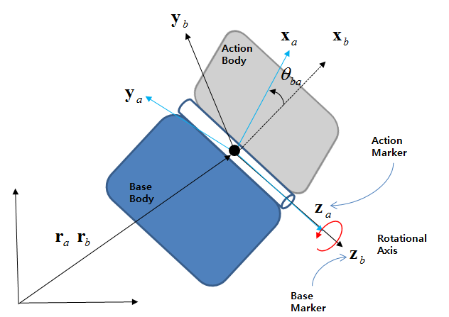
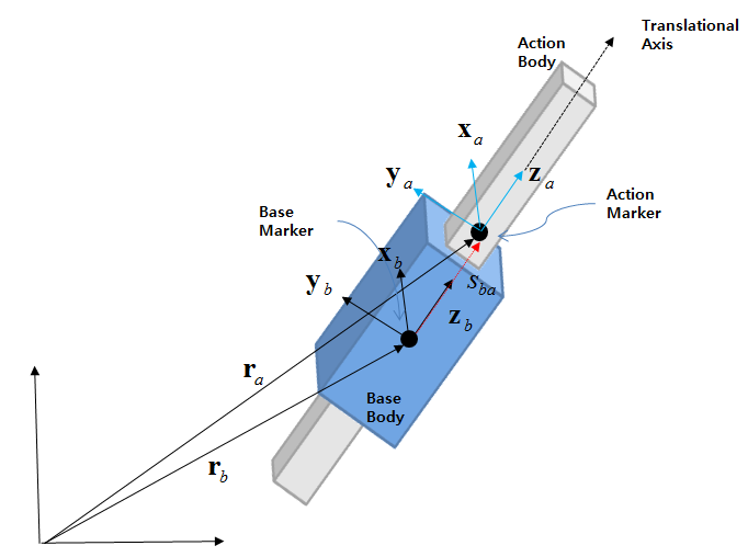
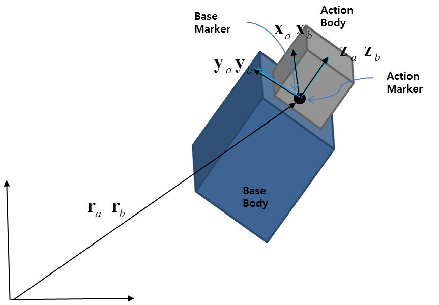
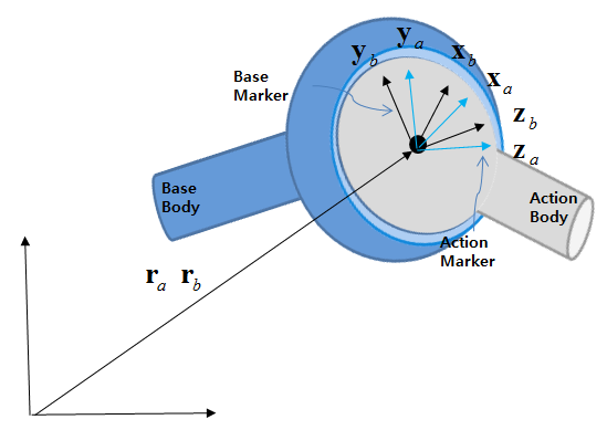
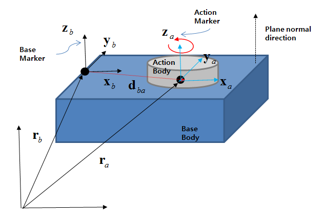
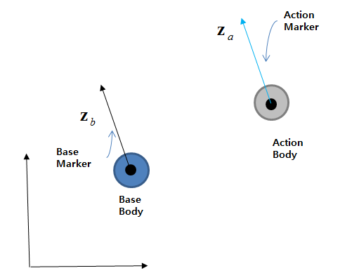
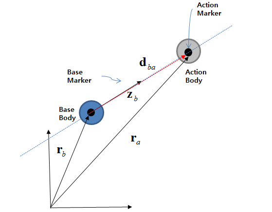
A Revolute Joint constrains three translational DOFs of one body relative to another body because the positions of two markers must be at the same location. The constraint equations of the position level can be represented using the following equations:
 | (5–1) |
where the vectors  and
and  are the absolute displacements of the action and base markers,
respectively. A revolute joint constrains two rotational DOFs of one body relative
to another body because the z-axes of the two markers must be parallel to the
rotational axis.
are the absolute displacements of the action and base markers,
respectively. A revolute joint constrains two rotational DOFs of one body relative
to another body because the z-axes of the two markers must be parallel to the
rotational axis.
The constraint equations of the position level can be represented using the following equations:
 | (5–2) |
where the vectors  ,
,  and
and  are the z-axis of the base marker and the x and y-axes of the
action marker, respectively.
are the z-axis of the base marker and the x and y-axes of the
action marker, respectively.
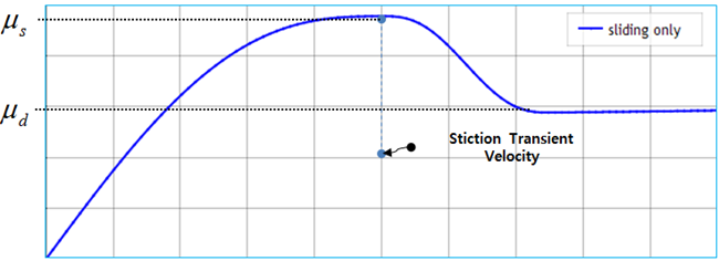
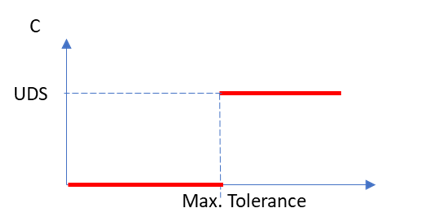
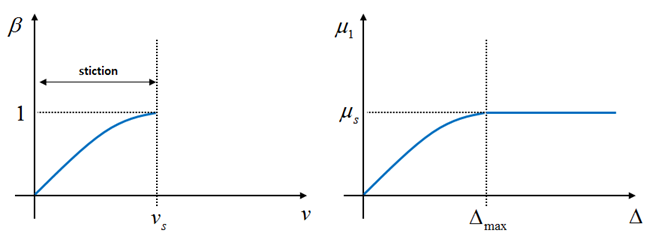
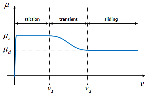
The dry friction which resists the relative motion between two contacted solids is subdivided into a static friction (or stiction) between non-moving surfaces and a kinetic friction (or sliding) between moving surfaces. The friction force can be represented by the Coulomb friction law as in following equation.
 | (5–3) |
where,  is a normal force and
  is a friction coefficient. The friction coefficient for the dry
friction can generally be taken from an experimental method and its pattern for the
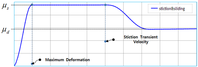
sliding velocity is similar to the figure below. The Motion solver uses the
pattern to get a friction coefficient in three regions refered to as stiction,
transient and sliding as shown in the figure below.
is a friction coefficient. The friction coefficient for the dry
friction can generally be taken from an experimental method and its pattern for the
sliding velocity is similar to the figure below. The Motion solver uses the
pattern to get a friction coefficient in three regions refered to as stiction,
transient and sliding as shown in the figure below.

In the figure,  and
and  are a static and dynamic friction coefficients taken from
experimental values.
are a static and dynamic friction coefficients taken from
experimental values.  and
and  are stiction and dynamic transient velocities, respectively. The
region is determined by a sliding velocity at a contact point between the contacted
surfaces and the sliding velocity can be calculated by the relative angular velocity
of
are stiction and dynamic transient velocities, respectively. The
region is determined by a sliding velocity at a contact point between the contacted
surfaces and the sliding velocity can be calculated by the relative angular velocity
of  and the pin radius of
  in the revolute joint as follows.
 | (5–4) |
When the sliding velocity is smaller than the stiction transient velocity, the friction coefficient can be calculated in the stiction range using the following equation:
 | (5–5) |

where  and
and  are the slip weight and slip friction coefficient, respectively.
 and
and  are the creep and the maximum deformation at the contact
point.
are the creep and the maximum deformation at the contact
point.
When the creep is greater than the maximum deformation, the slip friction coefficient is limited to the static friction coefficient. As shown in the figure above, the slip weight and friction coefficient can be calculated using STEP5 Function as in the following equations, respectively.
 | (5–6) |
 | (5–7) |
The creep  is a displacement moved under the stiction range and calculated
using the following equation:
is a displacement moved under the stiction range and calculated
using the following equation:
 | (5–8) |
where  is the starting angle of slip and is updated whenever the sliding
velocity comes into the stiction range from the transient or sliding range, as in
the figure Figure 5.2: Concept of friction coefficient. Initially, the
value is zero. When the friction effect option is defined as 2 or 3 in the
stiction range, the slip weight
is the starting angle of slip and is updated whenever the sliding
velocity comes into the stiction range from the transient or sliding range, as in
the figure Figure 5.2: Concept of friction coefficient. Initially, the
value is zero. When the friction effect option is defined as 2 or 3 in the
stiction range, the slip weight  or the slip friction coefficient
  become zero, respectively.
When the sliding velocity is greater than the stiction transient velocity and smaller than the dynamics transient velocity, the friction coefficient can be calculated by using STEP5 Function in the transient range as following equation.
 | (5–9) |
When the friction effect option is defined as 2 in
the transient range, the friction coefficient  becomes zero.
When the sliding velocity is greater than the dynamics transient velocity, the friction coefficient can be defined as the dynamics friction coefficient in the sliding range as in the following equation.
 | (5–10) |
When the friction effect option is defined as in 2
in the transient range, the friction coefficient  becomes zero.
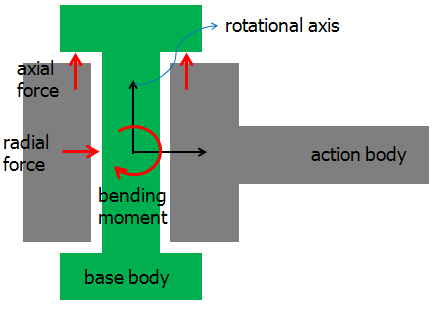
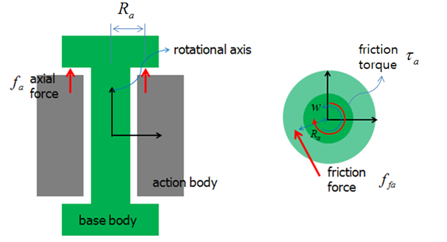
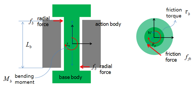
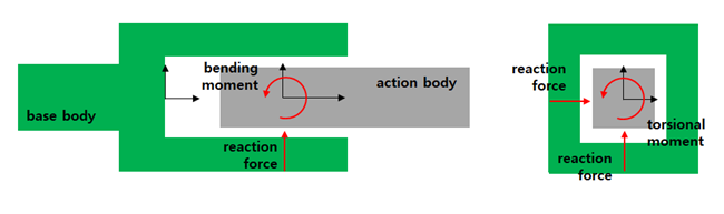
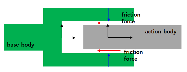
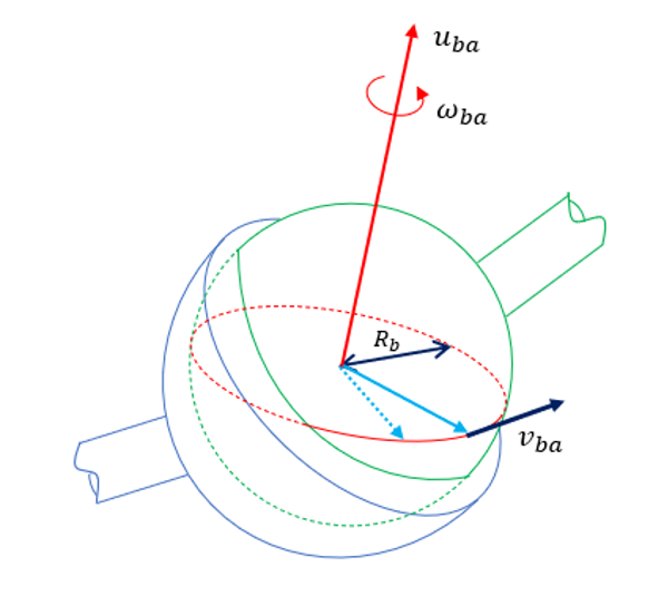
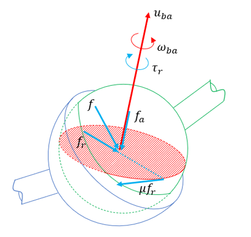
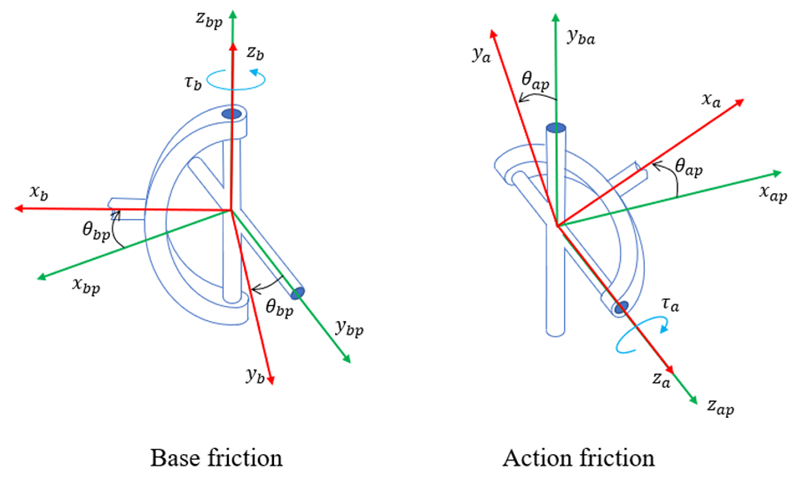
Constrained force and torque of the revolute joint can be subdivided into the axial force in the z-axis of the base marker, and the radial force and bending moment on the x-y plane of the base marker as shown in the figure below. Theses forces or torques can generate a friction force and then the friction force finally induces a resistant torque around the rotational axis.
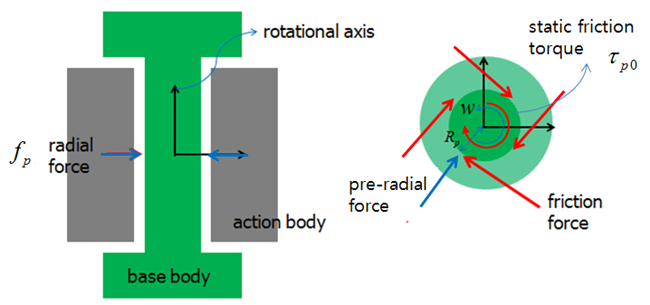
When the joint is under pre-loading, such as squeezing, as shown in the figure below, the friction torque must be considered as in the following equation:
 | (5–11) |
where  is the static torque due to the pre-friction force.
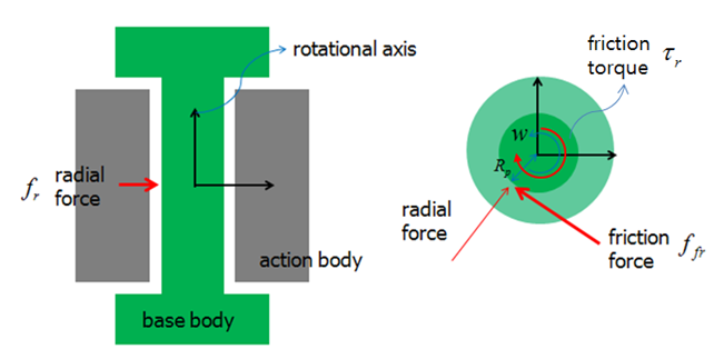
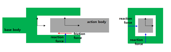
When a constrained force is applied at the joint in radial direction as shown in the figure below, the friction torque can be calculated using the following equation:
 | (5–12) |
where  and
and  are the pin radius and constrained force in the radial
direction.
are the pin radius and constrained force in the radial
direction.
When a constrained force is applied at the joint in axial direction as shown in the figure below, the friction torque can be calculated using the following equation:
 | (5–13) |
where  and
and  are the friction arm and constrained force in the axial
direction.
are the friction arm and constrained force in the axial
direction.
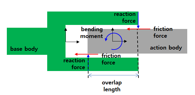
When the constrained force in the radial direction can disregarded due to force equilibrium, the bending moment may remain at the joint. In this case, the friction force for the disregarded radial forces is considered as shown in the figure below, and the friction torque can be calculated as in the following equation:
 | (5–14) |
where  ,
,  and
and  are the pin radius, bending reaction arm and constrained bending
moment in the radial direction.
are the pin radius, bending reaction arm and constrained bending
moment in the radial direction.
Total friction torque can be calculated using Equation 5–11 ~ Equation 5–14 as follows.
 | (5–15) |
When the Reaction Force option is cleared, the torques  and
and  become zero. When the Bending Moment option
is cleared, the torque
become zero. When the Bending Moment option
is cleared, the torque  becomes zero.
This friction torque is added to the constrained force from Equation 2–171 as follows.
 | (5–16) |
The definitions of parameters for the friction formulas are as shown in the table below.
Figure 5.9: Parameters for friction formulas in a revolute joint
| Symbol | Description | Dimension |
 | Static friction coefficient. This can be measured using an experimental method. | N/A |
 | Dynamic friction coefficient. This can be measured using an experimental method. | N/A |
 | Stiction transient velocity. This can be measured using an experimental method. | Length/Time |
 | Dynamic transient velocity. This can be measured using an experimental method. | Length/Time |
 | Maximum deformation under stiction. This affects the slip friction coefficient and can be determined artificially. | Length |
 | Pin radius. This affects the friction torque and can be determined geometrically. | Length |
 | Friction arm. This affects the friction torque due to the axial force and can be determined geometrically. | Length |
 | Bending reaction arm. This affects the friction torque due to the bending moment and can be determined geometrically. | Length |
STEP5 Function
The STEP5 function is one of the Heaviside step functions with a quintic polynomial. The usage of the function is same as for STEP and its formulas can be expressed as follows:

where
 and
and  .
.
Friction Effect
Friction coefficient pattern with sliding and stiction
When the creep approaches the maximum deformation under the stiction range, the friction coefficient approaches the static friction coefficient. Until the sliding velocity becomes the stiction transient velocity, the friction coefficient is retained as the static friction coefficient.
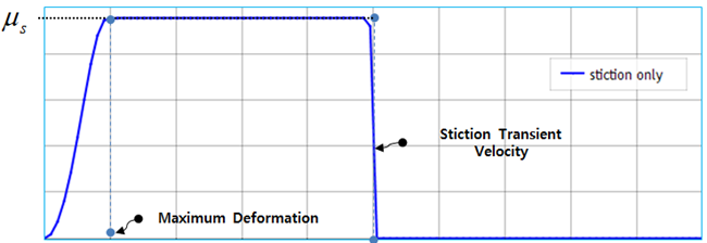
Friction coefficient pattern with stiction only
When the creep approaches the maximum deformation under the stiction range, the friction coefficient approaches the static friction coefficient. Until the sliding velocity becomes the stiction transient velocity, the friction coefficient is retained as the static friction coefficient. When the sliding velocity exceeds the stiction transient velocity, the friction coefficient becomes zero.
Friction coefficient pattern with sliding only
The friction coefficient is increased to the static friction coefficient as the sliding velocity under the stiction range. The friction coefficient is then determined by Equation 5–9 and Equation 5–10 under transient and sliding ranges, respectively.
If the joint doesn't have any Motion functions and
Restriction is enabled, the restriction torque for the revolute
joint  is calculated from the following equations.
 | (5–17) |
 | (5–18) |
If  is a positive value,
  and if
  is a negative value,
  .
.
In Equation 5–17,  and
and  are the stiffness and damping coefficients. The stiffness can be
calculated from the stiffness coefficient
are the stiffness and damping coefficients. The stiffness can be
calculated from the stiffness coefficient  and penetration of restriction p, as
follows.
and penetration of restriction p, as
follows.
 | (5–19) |
The damping coefficient can be calculated from the maximum damping  , and the boundary penetration,
  is the same as shown in Figure 6.63: Damping coefficient of contact force.
 and
and  are the relative angle and angular velocity of the action body
relative to the base body.
are the relative angle and angular velocity of the action body
relative to the base body.  are the positive and negative restriction angles defined by user
input in the Revolute Joint properties.
are the positive and negative restriction angles defined by user
input in the Revolute Joint properties.
If the joint has any Motion functions, the calculation of the restriction torque
 is not used. It is instead decided by the constraint equation that
restricts the motion.
is not used. It is instead decided by the constraint equation that
restricts the motion.
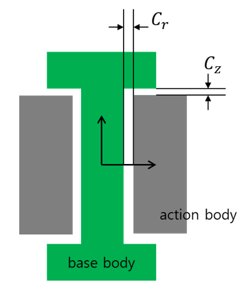
Clearance allows the relative displacement between the base and action markers of a joint to be as much as a defined value. When the relative displacement is greater than the clearance, a contact force is applied on the bodies. In a revolute joint, the clearance direction can be defined in the radial or axial direction as shown in the figure below.
When the joint clearance is defined, a constrained force on the joint will not work and is changed to a contact force. The force formula is calculated in the same way as for contact force. Contact detection is by the sign of penetration p. The penetration p can be calculated as follows:
 | (5–20) |
 | (5–21) |
where  is relative distance,
  is the unit vector of the contact direction such that
 is positive,
  is the relative displacement of the action marker with respect to
the base marker, and
is the relative displacement of the action marker with respect to
the base marker, and  is the clearance.
When calculating the clearance in the radial direction,  can be calculated as follows.
 | (5–22) |
 | (5–23) |
 | (5–24) |
 | (5–25) |
When calculating the clearance in the axial direction, un can be calculated as follows.
 | (5–26) |
When the sign of p is negative, the joint is not in contact. However, since the damping force by lubrication is effective, its force can be calculated as follows:
 | (5–27) |
where  is the damping coefficient and
  is the penetrating velocity.
The penetrating velocity  can be calculated using the following equation:
 | (5–28) |
where  is the relative velocity of the action marker with respect to the
base marker.
is the relative velocity of the action marker with respect to the
base marker.
When the sign of p is positive, the joint is in contact and the contact force can be calculated using the following equation:
 | (5–29) |
where  is the contact stiffness.
The contact stiffness can be calculated from the stiffness coefficient
 and the penetration using the following equation:
 | (5–30) |
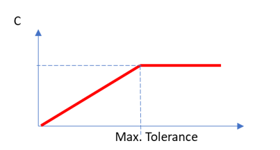
The damping coefficient can be calculated from the maximum damping cmax and clearance C. When the Damping effect in void option is selected, the damping coefficient can be calculated as shown in the figure and equation below.
 | (5–31) |
When Damping effect in void is not selected, the damping coefficient can be calculated as shown in the figure and equation below.
 | (5–32) |
The clearance forces are added to the constrained force as follows.
 | (5–33) |
(5–34) |
(5–35) |
Figure 5.14: Parameters for clearance formulas in a revolute joint
| Symbol | Description | Dimension |
| k | Stiffness coefficient. This stiffness and its exponent of deformation can be measured by experimental method or flexible body simulation. | Force/Length |
| n | Exponent of penetration. This and the stiffness coefficient can be measured by experimental method or flexible body simulation. When a body is slowly contacted with the other body, the deformation can be measured as increasing load is applied. From the curve of the load for the deformation, it is possible to estimate the stiffness coefficient and the exponent of penetration. | N/A |
| cmax | Maximum damping coefficient. This affects dynamic stiffness and can be measured by experimental method. | Force*Time/LengthTime |
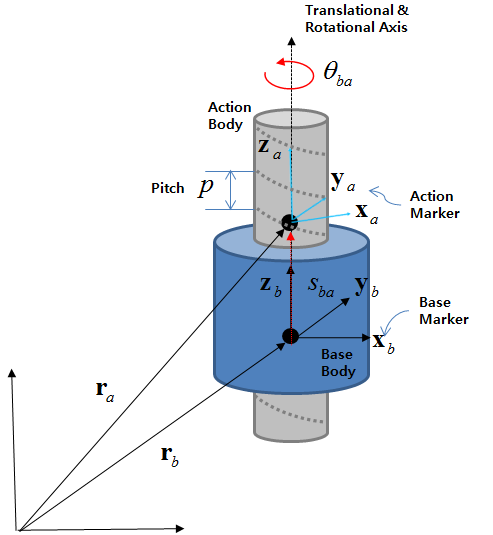
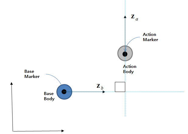
A Translational Joint constrains two translational DOFs of one body relative to another body because the location of the action marker must move along the z-axis of the base marker. The constraint equations of the position level can be represented by the following equations:
 | (5–36) |
where the vectors  and
and  are the absolute displacements of the action and base markers,
respectively. The vectors
are the absolute displacements of the action and base markers,
respectively. The vectors  and
and  are the x and y-axes of the base markers, respectively.
A translational joint constrains three rotational DOFs of one body relative to another body because the orientations of the two markers must be identical. The constraint equations of the position level can be represented by the following equations:
 | (5–37) |
where the vectors  ,
,  ,
,  and
and  are the z-axis of the base marker and the x, y and z-axes of the
action marker, respectively.
are the z-axis of the base marker and the x, y and z-axes of the
action marker, respectively.
The constrained forces are defined from Lagrange multipliers and can be written as follows.
 | (5–38) |
From Equation 5–19, the force in the translational axis direction becomes zero when coupler or motion is not added to the joint. The action force is applied to the action marker and an equal and opposite reaction force is applied to the base marker and the reaction torque due to the moment arm is added as follows.
 | (5–39) |
The dry friction which resists the relative motion between two solids in contact is subdivided into a static friction (or stiction) between non-moving surfaces and a kinetic friction (or sliding) between moving surfaces. The friction force can be represented by the Coulomb friction law using the following equation:
 | (5–40) |
where  is a normal force and
  is a friction coefficient.
The friction coefficient for dry friction can generally be taken by experimental method and its pattern for the relative velocity is similar to the figure below. The Motion solver uses this pattern to calculate a friction coefficient in three regions refered to as stiction, transient and sliding as shown in the figure below.

In the figure,  and
and  are static and dynamic friction coefficients taken by experimental
method.
are static and dynamic friction coefficients taken by experimental
method.  and
and  are stiction and dynamic transient velocities, respectively. The
region is determined by the sliding velocity at a contact point between contacted
surfaces and this sliding velocity can be calculated using the following
equation:
are stiction and dynamic transient velocities, respectively. The
region is determined by the sliding velocity at a contact point between contacted
surfaces and this sliding velocity can be calculated using the following
equation:
 | (5–41) |
where  and
and  are the z-axis of the base marker and the first time derivative of
the relative displacement between the two markers.
are the z-axis of the base marker and the first time derivative of
the relative displacement between the two markers.
When the relative velocity is smaller than the stiction transient velocity, the friction coefficient can be calculated in the stiction range using the following equation:
 | (5–42) |
where  and
and  are the slip weight and a slip friction coefficient, respectively.
 and
and  are the creep and the maximum deformation at the contact
point.
are the creep and the maximum deformation at the contact
point.
When the creep is greater than the maximum deformation, the slip friction coefficient is limited to the static friction coefficient. As shown in the figure above, the slip weight and friction coefficient can be calculated using STEP5 Function in the following equations, respectively.
 | (5–43) |
 | (5–44) |
The creep  is a displacement moved under the stiction range and calculated by
the following equation:
is a displacement moved under the stiction range and calculated by
the following equation:
 | (5–45) |
where  is the relative displacement of the action marker with respect to
the base marker and updated whenever the relative velocity comes into the stiction
range from the transient or sliding range in Figure 5.2: Concept of friction coefficient. Initially, the value is zero.
When the friction effect option is defined as 2, the slip weight becomes zero in
the stiction range. When the friction effect option is defined as in 3, the slip friction coefficient becomes zero in
the stiction range.
is the relative displacement of the action marker with respect to
the base marker and updated whenever the relative velocity comes into the stiction
range from the transient or sliding range in Figure 5.2: Concept of friction coefficient. Initially, the value is zero.
When the friction effect option is defined as 2, the slip weight becomes zero in
the stiction range. When the friction effect option is defined as in 3, the slip friction coefficient becomes zero in
the stiction range.
When the relative velocity is greater than the stiction transient velocity and smaller than the dynamic transient velocity, the friction coefficient can be calculated by using STEP5 Function in the transient range as in the following equation.
 | (5–46) |
When the friction effect option is defined as in 2
in the transient range, the friction coefficient  becomes zero.
When the relative velocity is greater than the dynamic transient velocity, the friction coefficient can be defined as the dynamic friction coefficient in the sliding range by the following equation.
 | (5–47) |
When the friction effect option is defined as in 2
in the transient range, the friction coefficient becomes
zero.
The constrained force and torque of the translational joint can be subdivided into the reaction force and the bending moment on the x-y plane of the base marker and torsional moment as shown in the figure below. These forces or torques can generate a friction force.
When the joint is under preload, such as squeezing, as shown in the figure below, the friction force must be considered as in the following equation:
 | (5–48) |
where  is the friction force under stationary state.
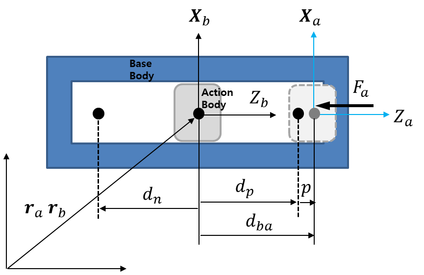
When a constrained force is applied in the x-y plane as shown in the figure below, the friction force from these reaction forces can be calculated by the following equation:
 | (5–49) |
where  is the constrained force in the x-y plane.
Though the constrained force in the x-y plane can be disregarded due to the force equilibrium, the bending moment may remain at the joint. In this case, the friction force for the disregarded reaction forces must be considered as shown in the figure below and can be calculated by the following equation:
 | (5–50) |
where  and
and  are the overlap length and constrained bending moment.
The three options in Motion for the overlap length are , , and .
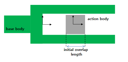
When the overlap length is constant as shown in the figure,  can be calculated using the following equation:
 | (5–51) |
where  is the initial overlap length.
When the overlap length increases while the action body moves in the positive z-axis
direction as shown in the figure below,  can be calculated from the following equation:
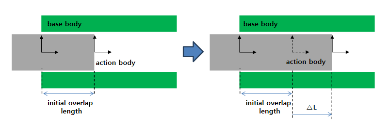
 | (5–52) |
where  is the change in relative displacement of the action marker with
respect to the base marker:
is the change in relative displacement of the action marker with
respect to the base marker:
 | (5–53) |
where  is the initial relative displacement of the action marker with
respect to the base marker.
is the initial relative displacement of the action marker with
respect to the base marker.
When the overlap length decreases while the action body moves in the positive z-axis
direction as shown in the figure below,  can be calculated from the following equation:
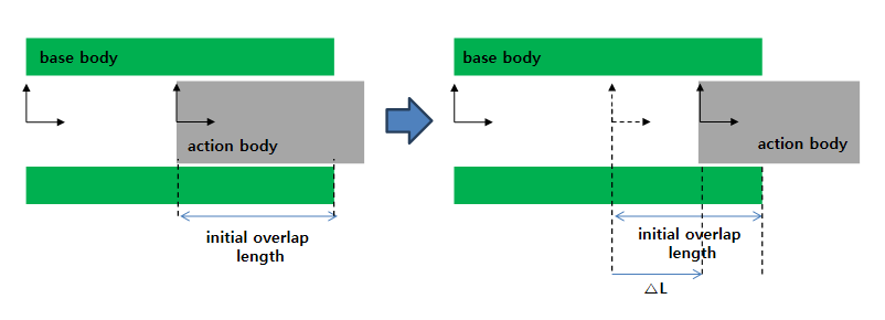
 | (5–54) |
Though the constrained force in x-y plane can be disregarded due to the force equilibrium, the torsional moment may remain at the joint. In this case, the friction force for the disregarded reaction forces is considered as shown in the figure below, and the friction force can be calculated as in the following equation:
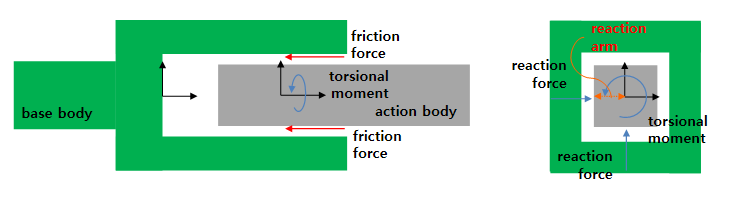
 | (5–55) |
where  and
and  are the reaction arm and constrained torsional moment.
Total friction force can be calculated with Equation 5–48 ~ Equation 5–55 as follows.
 | (5–56) |
When the Reaction Force option is not selected, the force
 becomes zero. When the Bending Moment option
is not selected, the force
becomes zero. When the Bending Moment option
is not selected, the force  becomes zero.
When the Torsional Moment option is not selected, the force  becomes zero.
These friction forces are added to the constrained force from Equation 5–39 as follows
 | (5–57) |
 | (5–58) |
The definitions of parameters for these friction formulas are as shown in the table below.
Figure 5.26: Parameters for friction formulas in a Translational Joint
| Symbol | Description | Dimension |
 | Static friction coefficient. This can be measured by experimental method. | N/A |
 | Dynamic friction coefficient. This can be measured by experimental method. | N/A |
 | Stiction transient velocity. This can be measured by experimental method. | Length/Time |
 | Dynamic transient velocity. This can be measured by experimental method. | Length/Time |
 | Maximum deformation under stiction. This affects the slip friction coefficient and can be determined artificially. | Length |
 | Friction arm. This affects the friction force due to the axial force and can be determined geometrically. | Length |
 | Bending reaction arm. This affects the friction torque due to the bending moment and can be determined geometrically. | Length |
If a joint doesn't have any Motion functions and restriction is enabled, the
restriction force of the translational joint,  is calculated by the following equations.
 | (5–59) |
 | (5–60) |
If  has a positive value, then
  . If
. If  has a negative value then
  .
.
 and
and  are the stiffness and damping coefficient. The stiffness can be
calculated from the stiffness coefficient
are the stiffness and damping coefficient. The stiffness can be
calculated from the stiffness coefficient  and the penetration of restriction
  as follows.
 | (5–61) |
The damping coefficient can be calculated from the maximum damping  , and the boundary penetration
  is the same as shown in Figure 6.63: Damping coefficient of contact force.
 ,
,  are the relative position and velocity of the action body with
respect to the base body.
are the relative position and velocity of the action body with
respect to the base body.  are the positive and negative restriction displacement defined by
user input in the translational joint properties.
are the positive and negative restriction displacement defined by
user input in the translational joint properties.
If the joint has any Motion functions, the calculation of the restriction force
 is not used. It is instead decided by the constraint equation used
to restrict the motion.
is not used. It is instead decided by the constraint equation used
to restrict the motion.
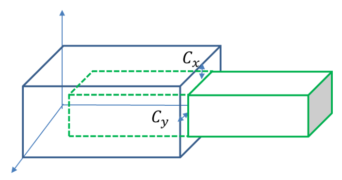
Clearance allows relative displacement between the base and action markers of a joint up to the defined value. When the relative displacement is greater than the clearance, a contact force is applied to the bodies. In a translational joint, the clearance direction can be defined in the x-axis and y-axis directions of the base marker as shown in the figure below.
The formulas for clearance in a translational joint are the same as that for a
revolute joint, but the definition of the clearance direction is different. When
calculating the clearance in the x direction,  can be calculated as in the following equation:
 | (5–62) |
When calculating the clearance in the y direction,  can be calculated as follows:
 | (5–63) |
A fixed joint constrains three translational DOFs of one body relative to another body because the location of the action marker must be locked at the same location as the base marker. The constraint equations at the position level can be represented by the following equation:
 | (5–64) |
where the vectors  and
and  are the absolute displacements of the action and base markers,
respectively.
are the absolute displacements of the action and base markers,
respectively.
A fixed joint constrains three rotational DOFs of one body relative to another body because the orientations of the two markers must be identical. The constraint equations at the position level can be represented by the following equation:
 | (5–65) |
where the vectors  ,
,  ,
,  ,
,  ,
,  and
and  are the x, y and z-axes of the base marker and the x, y and z-axes
of the action marker, respectively.
are the x, y and z-axes of the base marker and the x, y and z-axes
of the action marker, respectively.
The constrained forces are defined from Lagrange multipliers and can be written as follows.
 | (5–66) |
The action force is applied to the action marker and an equal and opposite reaction force is applied to the base marker as follows.
 | (5–67) |
A Ball Joint constrains three translational DOFs of one body relative to another body because the location of the action marker must be locked at the location of the base marker. The constraint at the position level can be represented by the following equation:
 | (5–68) |
where the vectors  and
and  are the absolute displacements of the action and base markers,
respectively. A Ball Joint does not constrain any rotational DOFs of one body
relative to another body because the relative rotations of the two markers must be
able to move freely. Consequently, there are no constraint equations.
are the absolute displacements of the action and base markers,
respectively. A Ball Joint does not constrain any rotational DOFs of one body
relative to another body because the relative rotations of the two markers must be
able to move freely. Consequently, there are no constraint equations.
The constrained forces are defined from Lagrange multipliers and can be written as follows.
 | (5–69) |
The action force is applied to the action marker and an equal and opposite reaction force is applied to the base marker as follows.
 | (5–70) |
A ball joint allows rotational motion relative to the x, y, and z-axes, but the friction torques are applied in the instantaneous direction of rotation. This direction is calculated from the relative angular velocity of the base body and the action body. The formula for the friction coefficient is same as that for a revolute joint. In a ball joint, the creep and the sliding velocity must be calculated on the instantaneous axis of rotation.
The creep Δ in the ball joint can be calculated by the following equation:
 | (5–71) |
where  is the relative rotation angle of relative orientation between the
base body and the action body in the previous time step and the current time
step.
is the relative rotation angle of relative orientation between the
base body and the action body in the previous time step and the current time
step.
The sliding velocity can be calculated by the relative angular velocity
 and the ball radius
  in the ball joint as follows:
 | (5–72) |
When the joint is under pre-loading, such as squeezing, as shown in the figure below, the friction torque must be considered as in following equation:
 | (5–73) |
where  is the static torque due to the pre-friction force.
The friction torque can be generated from just the radial force and is calculated using the following equation:
 | (5–74) |
where  is the ball radius.
Total friction torque can be calculated with Equation 5–57 and Equation 5–58 as follows.
 | (5–75) |
When the Reaction Force option is cleared, the torque
 becomes zero.
The definitions of the parameters for the friction formulas are as shown in the table below.
Figure 5.35: Friction formula parameters for a Ball Joint
| Symbol | Description | Dimension |
 | Relative rotation angle between previous and current steps. This is calculated from the Euler parameters of the change in relative orientation. | Radian |
 | Instantaneous axis of rotation. This is a unit vector of relative angular velocity. | N/A |
 | Ball radius. This affects the friction torque and can be determined geometrically. | Length |
A Cylindrical Joint constrains two translational DOFs of one body relative to another body because the location of the action marker must follow the z-axis of the base marker. The constraint equations at the position level can be represented as in the following equations.
 | (5–76) |
where, the vectors  and
and  are the absolute displacements of the action and base markers,
respectively. The vectors
are the absolute displacements of the action and base markers,
respectively. The vectors  and
and  are the x and y-axes of the base marker, respectively. A
Cylindrical Joint constrains two rotational DOFs of one body
relative to another body because the z-axes of the two markers must be parallel to
the rotational axis. The constraint equations at the position level can be
represented by the following equations.
are the x and y-axes of the base marker, respectively. A
Cylindrical Joint constrains two rotational DOFs of one body
relative to another body because the z-axes of the two markers must be parallel to
the rotational axis. The constraint equations at the position level can be
represented by the following equations.
 | (5–77) |
where, the vectors  ,
,  and
and  are the z-axis of the base marker and the x and y-axes of the
action marker, respectively. The constrained forces are defined from Lagrange
multipliers and can be written as follows.
are the z-axis of the base marker and the x and y-axes of the
action marker, respectively. The constrained forces are defined from Lagrange
multipliers and can be written as follows.
 | (5–78) |
From Equation 5–46, the force and torque in the rotational axis become zero when coupler or motion is not added to the joint. The action force is applied to the action marker and an equal and opposite reaction force is applied to the base marker and the reaction torque due to the moment arm is added as follows.
 | (5–79) |
A Plane Joint constrains one translational DOF of one body relative to another body because the location of the action marker must move on the x-y plane of the base marker. The constraint equations at the position level can be represented by the following equations:
 | (5–80) |
where the vectors  and
and  are the absolute displacements of the action and base markers,
respectively. The vector
are the absolute displacements of the action and base markers,
respectively. The vector  is the z-axis of the base markers.
A Plane Joint constrains two rotational DOFs of one body relative to another body because the z-axes of the two markers must be parallel to the normal direction. The constraint equations at the position level can be represented by the following equations:
 | (5–81) |
where the vectors  ,
,  and
and  are the z-axis of the base marker and the x and y-axes of the
action marker, respectively. The constrained forces are defined from Lagrange
multipliers and can be written as follows.
are the z-axis of the base marker and the x and y-axes of the
action marker, respectively. The constrained forces are defined from Lagrange
multipliers and can be written as follows.
 | (5–82) |
From Equation 5–46, forces on the x-y plane of the base marker and torque in the normal direction become zero. The action force is applied to the action marker and an equal and opposite reaction force is applied to the base marker and the reaction torque due to the moment arm is added as follows.
 | (5–83) |
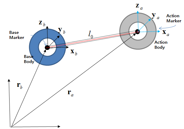
A Distance Joint constrains one translational DOF of one body relative to another body because the distance between the two markers must always be same as that specified. The constraint equations at the position level can be represented by the following equations.
 | (5–84) |
where, the vectors  and
and  are the absolute displacements of the action and base markers,
respectively. The constrained forces are defined from Lagrange multipliers and can
be written as follows.
are the absolute displacements of the action and base markers,
respectively. The constrained forces are defined from Lagrange multipliers and can
be written as follows.
 | (5–85) |
From Equation 5–53, the torques on the joint become zero. The action force is applied to the action marker and an equal and opposite reaction force is applied to the base marker and the reaction torque due to the moment arm is added as follows.
 | (5–86) |
A Universal Joint constrains three translational DOFs of one body relative to another body because the positions of the two markers must be at the same location. The constraint equations at the position level can be represented by the following equations.
 | (5–87) |
where, the vectors  and
and  are the absolute displacements of the action and base markers,
respectively. A Universal Joint constrains one rotational DOF
of one body relative to another body because the z-axes of the two markers must be
perpendicular. The constraint equations at the position level can be represented by
the following equations.
are the absolute displacements of the action and base markers,
respectively. A Universal Joint constrains one rotational DOF
of one body relative to another body because the z-axes of the two markers must be
perpendicular. The constraint equations at the position level can be represented by
the following equations.
 | (5–88) |
where, the vectors  and
and  are the z-axes of the base and action markers, respectively. The
constrained forces are defined from Lagrange multipliers and can be written as
follows.
are the z-axes of the base and action markers, respectively. The
constrained forces are defined from Lagrange multipliers and can be written as
follows.
 | (5–89) |
The action force is applied to the action marker and an equal and opposite reaction force is applied to the base marker and the reaction torque due to the moment arm is added as follows.
 | (5–90) |
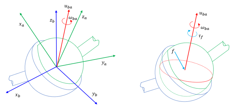
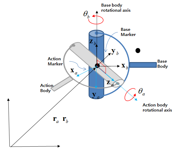
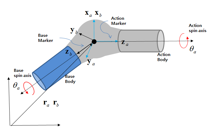
Universal joints support frictional torque in two rotational directions. A virtual crossed pin is internally generated to measure the relative angle and velocity in two rotational directions as shown in the figure below.
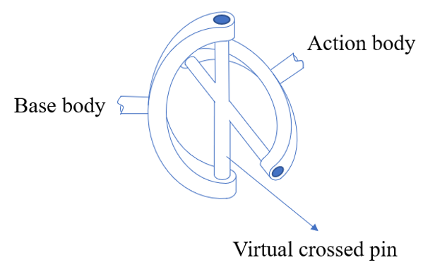
This allows the base and action bodies to rotate relative to the virtual crossed pin along the z-axes of the base and action markers of the joint. The frictional torques concerning relative rotational motion can be calculated with the relative angles and rotational velocities of the base body or action body with respect to the virtual crossed pin. The formulas for frictional torque in each rotational direction are the same as for Friction in a Revolute Joint.
The kinematic constraint equations of a Screw Joint are exactly same as for a Cylindrical Joint, but this joint has an additional constraint between relative displacement and angle.
The pitch defines the amount of translational displacement of the two markers for every rotation about the rotation axis as in the following equation:
 | (5–91) |
where  is the value of the pitch.
  and
and  are the relative displacement in Equation 5–37 and
angle in Equation 2–165, respectively. If the screw is a right-handed
thread, the pitch value must be positive. Otherwise, if the screw is a left-handed
thread, the pitch value must be negative.
are the relative displacement in Equation 5–37 and
angle in Equation 2–165, respectively. If the screw is a right-handed
thread, the pitch value must be positive. Otherwise, if the screw is a left-handed
thread, the pitch value must be negative.
The constrained forces are defined from Lagrange multipliers and can be written as follows.
 | (5–92) |
From Equation 5–64, the force and torque in the z-axis direction of the base marker will create the necessary force and torque to satisfy the constraint equation Equation 5–48. The action force is applied to the action marker and an equal and opposite reaction force is applied to the base marker and the reaction torque due to the moment arm is added as follows.
 | (5–93) |
Note: Since, from Equation 2–165 for a revolute joint, this entity can cause a problem during solving when the rotating angle exceeds π in a single time step, the Motion solver may display a warning message in the message file under dynamic analysis. The warning condition is when the rotational velocity * step size is bigger than π. In this case, you must set the maximum step size to a smaller value in order to avoid the problem. This situation only occurs when a body rotates at extreme speeds.
A Constant Velocity Joint constrains three translational DOFs of one body relative to another body because the positions of the two markers must be at the same location. The constraint equations at the position level can be represented by the following equation:
 | (5–94) |
where the vectors  and
and  are the absolute displacements of the action and base markers,
respectively. A Constant Velocity Joint constrains the
rotational DOFs of each body because angular velocities in the z-axes of the two
markers must be equal.
are the absolute displacements of the action and base markers,
respectively. A Constant Velocity Joint constrains the
rotational DOFs of each body because angular velocities in the z-axes of the two
markers must be equal.
The constraint equations at the velocity level can be represented by the following equation:
 | (5–95) |
where the vectors  ,
,  ,
, and
and  are the z-axes of the base and action markers and the angular
velocities of the base and action bodies, respectively.
are the z-axes of the base and action markers and the angular
velocities of the base and action bodies, respectively.
The constrained forces are defined from Lagrange multipliers and can be written as follows.
 | (5–96) |
The action force is applied to the action marker and an equal and opposite reaction force is applied to the base marker as follows.
 | (5–97) |
An Orientation Primitive constrains three rotational DOFs of one body relative to another body because the orientations of the two markers must be the same. The constraint equations at the position level can be represented by the following equations:
 | (5–98) |
where the vectors  ,
,  ,
,  and
and  are the z-axis of the base marker and the x, y and z-axes of the
action marker, respectively. The constrained forces are defined from Lagrange
multipliers and can be written as follows.
are the z-axis of the base marker and the x, y and z-axes of the
action marker, respectively. The constrained forces are defined from Lagrange
multipliers and can be written as follows.
 | (5–99) |
The action force is applied to the action marker and an equal and opposite reaction force is applied to the base marker as follows.
 | (5–100) |
A Parallel Primitive constrains two rotational DOFs of one body relative to another body because the z-axes of two markers must be parallel. The constraint equations at the position level can be represented by the following equations:
 | (5–101) |
where the vectors  ,
,  , and
, and  are the z-axis of the base marker and the x and y-axes of the
action marker, respectively.
are the z-axis of the base marker and the x and y-axes of the
action marker, respectively.
The constrained forces are defined from Lagrange multipliers and can be written as follows.
 | (5–102) |
The action force is applied to the action marker and an equal and opposite reaction force is applied to the base marker as follows.
 | (5–103) |
An Inline Primitive constrains two translational DOFs of one body relative to another body because the location of the action marker must move along the straight line defined by the z-axis of base marker. The constraint equations at the position level can be represented by the following equations:
 | (5–104) |
where the vectors  ,
,  ,
,  and
and  are the x and y-axes of the base marker and the absolute
displacements of the action and base markers, respectively.
are the x and y-axes of the base marker and the absolute
displacements of the action and base markers, respectively.
The constrained forces are defined from Lagrange multipliers and can be written as follows.
 | (5–105) |
The action force is applied to the action marker, an equal and opposite reaction force is applied to the base marker and the reaction torque due to the moment arm is added as follows.
 | (5–106) |

An Inplane Primitive constrains one translational DOF of one body relative to another body because the location of action marker must move on the x-y plane of the base marker. The constraint equations of the position level can be represented by the following equations:
 | (5–107) |
where the vectors  ,
,  and
and  are the z-axis of the base marker and the absolute displacements
of the action and base markers, respectively.
are the z-axis of the base marker and the absolute displacements
of the action and base markers, respectively.
The constrained forces are defined from Lagrange multipliers and can be written as follows.
 | (5–108) |
The action force is applied to the action marker, an equal and opposite reaction force is applied to the base marker and the reaction torque due to the moment arm is added as follows.
 | (5–109) |
A Perpendicular Primitive constrains one rotational DOF of one body relative to another body because the z-axes of the two markers must be perpendicular. The constraint equations at the position level can be represented by the following equations:
 | (5–110) |
where the vectors  and
and  are the z-axes of the base and action markers,
respectively.
are the z-axes of the base and action markers,
respectively.
The constrained forces are defined from Lagrange multipliers and can be written as follows.
 | (5–111) |
The action force is applied to the action marker and an equal and opposite reaction force is applied to the base marker as follows.
 | (5–112) |
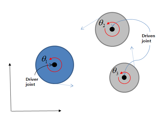
A Coupler constrains the relative translational or/and rotational motions of two or three joints. For example, when three revolute joints are coupled, the constraint equations of the position level can be represented by the following equation:
 | (5–113) |
where  ,
,  and
and  are scale factors to define a motion ratio between the
joints.
are scale factors to define a motion ratio between the
joints.
The constrained force or torque is defined from Lagrange multipliers and it is added to the force or torque of each joint.
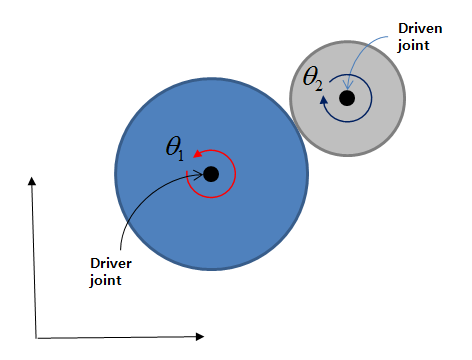
A Gear constrains the relative rotational motion of two joints. The constraint equations at the position level can be represented by the following equation:
 | (5–114) |
where  and
and  are scale factors to define the motion ratio between
joints.
are scale factors to define the motion ratio between
joints.
The constrained torque is defined from Lagrange multipliers and it is added to the torque of each joint.
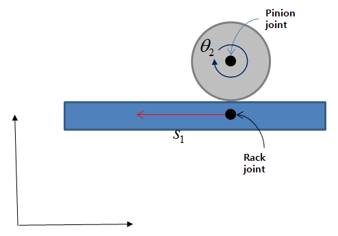
A Rack and Pinion constrains the relative motions of two joints. The constraint equations at the position level can be represented by the following equation:
 | (5–115) |
where  and
and  are scale factors to define the motion ratio between the
joints.
are scale factors to define the motion ratio between the
joints.
The constrained force and torque are defined from Lagrange multipliers and they are added to the force and torque of each joint.
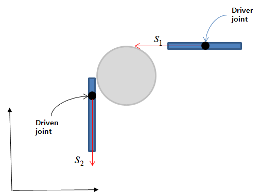
A Cable constrains the relative translational motions of two joints. The constraint equations at the position level can be represented by the following equation:
 | (5–116) |
where  and
and  are scale factors to define the motion ratio between the
joints.
are scale factors to define the motion ratio between the
joints.
The constrained force is defined from Lagrange multipliers and it is added to the force of each joint.
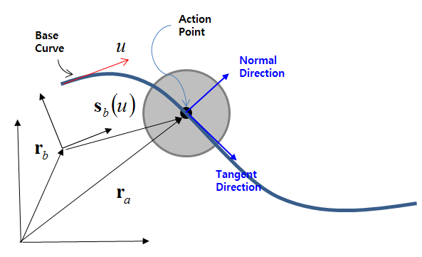
A PTCV object has one additional degree of freedom for the floating point on the curve of the base body, and the floating point and the fixed point on the action body are constrained to lie on the same position.
The constraint equations at the position level can be represented by the following equation:
 | (5–117) |
where the vectors  ,
,  , and
, and  are the positions of the base marker, the floating point of curve,
and the action marker, respectively. The position of the floating point on the curve
is calculated by using the Interpolation Functions in Curveset as a Connector for Constraints.
are the positions of the base marker, the floating point of curve,
and the action marker, respectively. The position of the floating point on the curve
is calculated by using the Interpolation Functions in Curveset as a Connector for Constraints.
The constrained forces are defined from the penalty method and can be written as follows.
 | (5–118) |
The action force is applied to the action marker and an equal and opposite reaction force is applied to the base floating marker as follows.
 | (5–119) |
A PTCV object allows the action marker to have a purely
sliding motion relative to the curve on the base marker. The sliding
displacement  can be defined as follows:
 | (5–120) |
where  and
and  are the current and initial geometric parameters of the
floating point on the base curve.
are the current and initial geometric parameters of the
floating point on the base curve.
The sliding velocity and acceleration can be represented by the following equations.
 | (5–121) |
 | (5–122) |
Thus, the driving constraint equations in the velocity and acceleration levels can be defined with the sliding displacement and its time derivatives of Equation 5–100 ~ Equation 5–102 as follows:
 | (5–123) |
 | (5–124) |
where the function  can be defined by a Function Expression
or Motion User Subroutine. The function can be dependent on
the displacement, velocity, and acceleration of other bodies, variable and
differential equations, and time.
can be defined by a Function Expression
or Motion User Subroutine. The function can be dependent on
the displacement, velocity, and acceleration of other bodies, variable and
differential equations, and time.
The driving torque is defined from Lagrange multiplier and added to the constrained force from Equation 5–98 as follows:
 | (5–125) |
where the driving force  is a force in the tangential direction of the curve. This
force corresponds to the force necessary to slide the action body relative to
the base body.
is a force in the tangential direction of the curve. This
force corresponds to the force necessary to slide the action body relative to
the base body.
The dry friction which resists the sliding motion between the action point and the base curve is subdivided into a static friction (or stiction) between a non-moving curve and a kinetic friction (or sliding) between a moving curve. The friction force can be represented by the Coulomb friction law as in following equation:
 | (5–126) |
where,  is the normal force and
  is the friction coefficient. The friction coefficient for the
dry friction can generally be taken from an experimental method.
is the friction coefficient. The friction coefficient for the
dry friction can generally be taken from an experimental method.
The Motion solver uses the pattern to get a friction coefficient in three regions refered to as stiction, transient and sliding as shown in the figure below.
In the figure above,  and
and  are the static and dynamic friction coefficients taken from
experimental values.
are the static and dynamic friction coefficients taken from
experimental values.  and
and  are stiction and dynamic transient velocities, respectively. The
region is determined by the sliding velocity
are stiction and dynamic transient velocities, respectively. The
region is determined by the sliding velocity  in Equation 5–101 as follows.
 | (5–127) |
The friction coefficient can be calculated using the sliding velocity in Friction in a Revolute Joint in Equation 5–5 ~ Equation 5–10. Finally, the friction force from Equation 5–106 is added to the constrained force from Equation 5–105 in the tangential direction.
A CVCV object has two additional degrees of freedom for the floating points on the two curves of the action and base bodies, and two floating point are constrained to lie at the same position. The constraint equations at the position level can be represented by the following equations.
 | (5–128) |
where, the vectors  ,
,  ,
,  , and
, and  are the positions of the base marker, the floating point of the
base curve, the action marker, and the floating point of the action curve,
respectively. The positions of the floating points on the curves are calculated by
using the Interpolation Functions in Curveset as a Connector for Constraints. The action and base curves must both be planar curves. The Motion solver
initially calculates the plane normal vectors
are the positions of the base marker, the floating point of the
base curve, the action marker, and the floating point of the action curve,
respectively. The positions of the floating points on the curves are calculated by
using the Interpolation Functions in Curveset as a Connector for Constraints. The action and base curves must both be planar curves. The Motion solver
initially calculates the plane normal vectors  and
and from the passing points of each curve. Then, the plane normal
vectors are constrained to be parallel in the time domain using the following
equations.
from the passing points of each curve. Then, the plane normal
vectors are constrained to be parallel in the time domain using the following
equations.
 | (5–129) |
where, the vectors  and
and  are the arbitrary vectors which are orthogonal to the plane normal
vector of the action curve.
are the arbitrary vectors which are orthogonal to the plane normal
vector of the action curve.
The constrained forces are defined from the penalty method and can be written as follows.
 | (5–130) |
The action force is applied to the action floating marker and an equal and opposite reaction force is applied to the base floating marker as follows.
 | (5–131) |
CVCV allows that the action floating marker has a purely sliding
motion relative to the base curve. The sliding displacement  can be defined as follows.
 | (5–132) |
where,  ,
,  ,
,  , and
, and  are the current and initial geometric parameters of the action and
base floating points. The sliding velocity and acceleration can be represented by
the following equations.
are the current and initial geometric parameters of the action and
base floating points. The sliding velocity and acceleration can be represented by
the following equations.
 | (5–133) |
The dry friction which resists the sliding motion between curves is subdivided into static friction (or stiction) between non-moving curves and kinetic friction (or sliding) between moving curves. The friction force can be represented by the Coulomb friction law as in the following equation.
 | (5–134) |
where,  is the normal force and
  is the friction coefficient. The friction coefficient for the dry
friction can generally be taken from an experimental method. The Motion solver
uses the pattern to get a friction coefficient in three regions refered to as
stiction, transient and sliding as shown in Figure 5.54: Concept of Friction Coefficient.
is the friction coefficient. The friction coefficient for the dry
friction can generally be taken from an experimental method. The Motion solver
uses the pattern to get a friction coefficient in three regions refered to as
stiction, transient and sliding as shown in Figure 5.54: Concept of Friction Coefficient.
The friction coefficient can be calculated using the sliding velocity in Friction in a Revolute Joint in Equation 5–5 ~ Equation 5–10. Finally, the friction force in Equation 5–114 is added to the constrained force from Equation 5–110 in the tangential direction.
A SixMotion object defines the relative three translational and three rotational motion DOFs for one body with respect to another body.
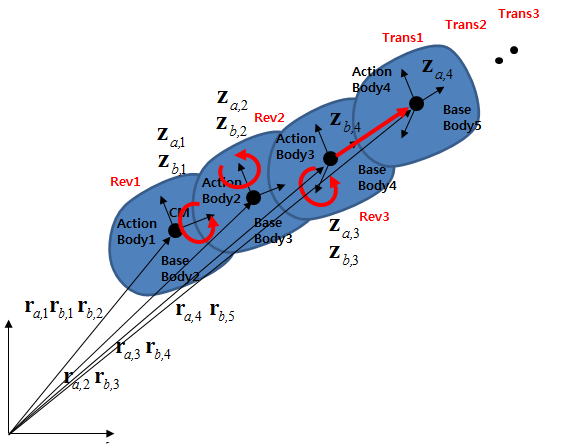
There are 5 dummy bodies in same position, so three Revolute Joint and three Translational Joint objects are connected to each dummy body as shown in the figure above.
The first revolute joint is applied to the x-axis direction between ground and the first dummy body. The second revolute joint is applied to the y-axis direction between the first dummy body and the second dummy body. A further revolute joint and three translational joints are connected using the same method.