


This option enables the transfer of stresses, strains, and history variables between solid meshes. Additionally, it enables repositioning the history variables as needed.
This section covers the following topics:
- 4.3.1. Main Mapping Command
- 4.3.2. Input and Output Meshes
- 4.3.3. Target Part IDs and Source Part IDs
- 4.3.4. Transformation Options
- 4.3.5. Mapping Options
- 4.3.6. Equation Parser
- 4.3.7. Clustering Methods
- 4.3.8. Workflow with MAT_TAUGHENED_ADHESIVE_POLYMER Material Model
- 4.3.9. Output: Initial Stress Cards
- 4.3.10. Output: New *PART and *MAT252 Cards
- 4.3.11. Mapping
- 4.3.12. Commands
| SourceFile = STRING | Define the name and, if needed, the path of the source file (usually a *.dynain file). |
| TargetFile = STRING | Define the name and, if needed, the path of the target file. The target file must be an LS-DYNA application mesh. |
| MappingResult = STRING | Define the result file name. The mapping result is written into this newly generated file. |
|
OrientationFile = HISV Nodes | To enable the transfer of orientations, define this flag. It informs the program that the orientation data is stored within the history variables (HISV). Alternatively, you have the option of deriving the orientations from the element nodes. This method may yield accurate results if the mesh is well-aligned initially. |
| TransformedMeshFile = STRING | Specify the file name where the transformed mesh is written. This option is intended solely for postprocessing of the transformation. For additional details, refer to the Transformation Options section below. |
| AddEleHISVFile# = STRING | A file name carrying element histories in an additional file. Multiple of these files can be defined. The first 10 digits of the lines must hold the element ID, the following 10 digits carry some arbitrary value, interpreted as an additional history variable on the element level. |
| LookupTable# = STRING | A file name carrying lookup tables. Values within one line are separated by a space. As described in the Equation Parser section, the Envyo application enables history variable lookup based on these looktables provided by you. Following the lookup table command, you must define the columns that are considered for variable lookup. See the example in the Equation Parser section. |
The following options are available for the source, target, and result file formats:
|
SourceFileFormat = LS-DYNA ESI-PC Nastran HDF5 ESI-HDF5 GCODE ABAQUS STEP CSV | The source file format. The preferred format is LS-DYNA. |
| TargetFileFormat = LS-DYNA | The target file format. The only format available is LS-DYNA. |
| ResultFileFormat = LS-DYNA | The result file format. The only format available is LS-DYNA. |
| NumTargetPids = INT |
Define the number of parts in the target mesh which are considered within the mapping. This option must be followed by TargetPid#i definitions. |
| TargetPid#i = INT | Define as many part IDs as given in NumTargetPids. These parts are considered for the mapping. |
| NumSourcePIDs = INT |
Define the number of parts in the source mesh which are considered within the mapping. This option must be followed by SourcePID#i definitions. |
| SourcePID#i = INT | Define as many part IDs as given in NumSourcePIDs. These parts are considered for the mapping. |
Note: The options above specifically narrow down the scope of the mapping procedure to defined-part IDs. Other parts are ignored on both the source and target meshes.
|
TRANSFORMATION = YES NO | Turn the transformation option on or off. |
|
WriteTransformedMesh = YES NO | Flag to enable output of the transformed mesh used for mapping. This enables verifying the success of the transformation. If set to YES, a TransformedMeshFile must be specified (see Input and Output Meshes). |
There are three available methods for performing mesh transformation:
TRAFO_OPTION is required:
Iterative Closest Point (ICP)
Four-Points-Congruent Sets (4PCS)
TRAFO_OPTION is not required:
User-defined translation and rotation
The 4PCS method must be used with caution, as it is fully automatic and may not accurately transform stress tensors and fiber orientations between different coordinate systems. The ICP algorithm is the recommended approach.
The user-defined translation and rotation options are listed underneath TRAFO_OPTION.
Note: Transformation options are used to transform the source mesh.
|
TRAFO_OPTION = 4PCS ICP | Flag that enables specification of the desired transformation option. |
| NodalPair#i = INT INT | Define nodal pairs to initialize mesh alignment for the ICP algorithm. You may specify up to ten nodal pairs, with a minimum of three required. In each pair, the first integer represents a node ID in the source mesh, and the second corresponds to a node ID in the target mesh. Input values must be space-separated, with each nodal pair provided on a separate line. |
| MAX_NUM_ITER = INT | Maximum number of iterations to be performed by the 4PCS algorithm. |
| GLOBAL_ERR = DOUBLE | Global error measure to accept transformation as best fit 4PCS algorithm. |
| MATCHING_POINT_DIST = DOUBLE |
Maximum distance between points so that they are accepted as matching (4PCS). |
| PERCENTAGE_OF_MATCHING_POINTS = DOUBLE | Percentage of matching points to accept the transformation (4PCS). |
Additionally, a custom sequence of user-defined transformations can be applied. These transformations are executed in the order in which they are specified and multiple transformations may be defined:
|
RotateSRC = DOUBLE;X DOUBLE;Y DOUBLE;Z DOUBLE; DOUBLE DOUBLE DOUBLE | The source mesh rotates by a specified angle (first value, in degrees) around a defined axis. Predefined axes include X, Y, and Z. Alternatively, a custom axis can be specified by providing three space-separated floating-point values following a semicolon (; x y z). |
| MoveSRC = DOUBLE DOUBLE DOUBLE | The source mesh moves along the user-defined vector (x y z). |
| ScaleSRC = DOUBLE | The source mesh scales around the origin using the defined scale factor. |
In addition to the transformation options, there are options to convert the unit systems:
|
ChangeUnitSystem = YES NO | Activates or deactives unit system conversion. |
|
SourceUnitSystem = kg - m - s ton - mm - s kg - mm - ms g - mm - ms lb - in - s | If the unit system conversion is activated, provide information about the source unit system. |
|
TargetUnitSystem = kg - m - s ton - mm - s kg - mm - ms g - mm - ms lb - in - s | If the unit system conversion is activated, provide information about the target unit system. |
| ALGORITHM = ClosestPoint | The only available option is ClosestPoint. Values are mapped to the nearest node, integration point, or element center. |
|
Search_Radius = SrcEleLen TarEleLen DOUBLE | Specifies the search radius for the mapping algorithm. By default, SrcEleLen is used, which sets the radius to the average element size of the source mesh. Alternatively, you can use TarEleLen to apply the average element size of the target mesh, or provide a positive DOUBLE value to define a custom radius. |
| Scale_SearchRadius = DOUBLE | Coefficient to scale search radius. The default value is 1.0. |
| ETYP = INT |
1 - Reduced integrated solid elements. 2 - Fully integrated solid elements. |
|
MapStress = YES NO | Activates or deactivates stress mapping. |
|
MapStrain = YES NO | Activates or deactivates strain mapping. |
| InitialStress = DOUBLE | Enables initializing a specific stress value for all elements and integration points. This flag is mainly used to remove all stresses after mapping is performed, so that InitialStress = 0.0. |
|
HISV_HANDLING = YES NO CLEAR | Enables moving and modifying history variables with custom definitions. Regarding the meaning of histories, refer to [20], [4]. If CLEAR, all history variables are removed before generating the result file. If YES, define as many history variables as must be modified in the following way: |
| MAX_NUM_HISV = INT | Define a new maximum number of history variables. This is an easy way to get rid of unwanted histories which are not useful for the new model, but also enables extending the amount of histories being output. If a history variable is being moved to a position which is higher than the actual number of history variables in the input deck, the number of histories are extended automatically. |
| STRESS TENSOR POS = INT | Position of the beginning of the stress tensor, if stored on history variables. |
| SORT = BUCKET | Using bucket sort is strongly recommended, as it provides a substantial performance improvement for the search algorithm. |
| REPEAT = YES | Enable this option to ensure that all elements and integration points receive mapped data. When there is a significant difference in element sizes between the source and target meshes, the default bucket refinement may be insufficient to cover all points, sometimes by design. In such cases, this flag must be set to guarantee complete data coverage. |
The Envyo application implements an equation parser based on the Shunting yard algorithm and is available as MIT license [6]. This equation parser is modified to work with common variables in the LS-DYNA application such as histories, eff. plast. strains, and stresses. Variables are declared, using the & symbol and commands are executed in the order of input. The following variables are available:
| &HISV#i | History variable at position i. |
| &EPS | Effective plastic strain (the last entry in *INITIAL STRESS SHELL which may have a different meaning than eff. plast. strain). |
| &ELELENGTH | Element length of the current element. |
| &SIG_IJ | Components of the second order stress tensor. |
| &SIG_INIT | Enables initializing a specific stress value that refers to all stress components. |
| &ADD ELE HISV#i | Element history variable from file i is used. |
| &LookupTable#i | Lookup table from file i is used. |
| exp | Exponent. An alternative input is e**. |
The following example illustrates the usage of the equation parser in combination with the lookup tables. The commands following the additional history and lookup table definition are executed in the order of input.
Example of History Variable Manipulation
 AddEleHISVFile#1 = Results A.dyn
 AddEleHISVFile#2 = Results B.dyn
 LookupTable#1 = data A.txt,&COL#1,&COL#2,&COL#3
 LookupTable#2 = data B.txt,&COL#1,&COL#2,&COL#3
 &HISV#3 = &ADDELE HISV#2
 &HISV#2 = &ADDELE HISV#1
 &HISV#4 = abs(&HISV#3-&HISV#2)*0.000467354
 &EPS = &LookupTable#1,linearInterpolation,&HISV#4,&ELELENGTH,&COL#3
 &HISV#6 = &LookupTable#2,nextNeighbour,&EPS,&ELELENGTH,&COL#3
 &HISV#8 = &HISV#2
 &HISV#9 = &ELELENGTH MAX_NUM_HISV = 8
Two additional element history files are loaded into the Envyo application, and are stored internally. Additionally, two lookup table files are read. Columns one, two, and three are considered for both files. The column numbers can be different, and the lookup tables may have more than three columns. After reading the data, the following commands are executed:
Additional element history variable from file 2 is stored as history variable #3. Additional element history variable from file 1 is stored as history variable #2. The value of history variable #4 is calculated by multiplying the absolute value of history #3-#2 with a scale factor.
To get information about the eff. plastic strain, lookup table #1 is used. If values are inbetween two values provided within one of the columns, linear interpolation is used. In this case, history variable #4 is compared to values stored in column #1. Following that, Envyo takes the element length of each element, and compares it with the values stored in column #2 of lookup table #1. The final result is the value provided in column #3.
The value of history variable #6 is derived in a comparable way, considering the next neighbor instead of performing a linear interpolation between the values. The first input is the resulting eff. plastic strain from the previous step. Again, results are provided in column #3.
Following these operations, history variable #8 is assigned the value at history variable #2, and the element length is stored at history variable #9. Nevertheless, only eight history variables are written to the final result file due to MAX_NUM_HISV.
Part clustering is available on arbitrary history variables or even stress values. The input is as follows:
CLUSTERID#i = STRING, STRING, DOUBLE, DOUBLE, INT (,INT)
The value at i refers to the old part ID in the target mesh.
The first STRING refers to the history variable or stress component which is used for part clustering (see the Equation Parser section).
The second STRING refers to the clustering method. Possible inputs are AVG for average or MinMax. In any case, the average of the values stored on integration points is used for evaluation.
The DOUBLE values refer to the values to which the averaged component (first STRING) is compared to. If AVG is defined, comparison uses these exact intervals. If the MinMax option is chosen, these values are the overall range of history variable values that are split into equally-spaced intervals by the provided optional (last) INT value. The first DOUBLE value refers to .GE., the second DOUBLE value to .LT.
The following INT value refers to the assigned part ID after clustering. If the MinMax option is chosen, this is the starting part ID for the lowest equally-spaced range.
The last INT value is only required for the MinMax option, and defines the number of equally-spaced splits to be performed.
Example
CLUSTERID#500004 = &HISV3,MinMax,1.248,9.120E+02,12,6
Target part ID 500004 is split based on history variable #3. The MinMax option is chosen, therefore, internally, the Envyo application creates 6 equally spaced regions between 1.248 and 9.12E+02. Averaged values of history variable #3 are assigned part IDs starting at part ID 12.
CLUSTERID#500004 = &HISV3,AVG,1.248,2.803E+02,12
CLUSTERID#500004 = &HISV3,AVG,2.803E+02,4.067E+02,13
CLUSTERID#500004 = &HISV3,AVG,4.067E+02,5.330E+02,14
CLUSTERID#500004 = &HISV3,AVG,5.330E+02,6.593E+02,15
CLUSTERID#500004 = &HISV3,AVG,6.593E+02,8.857E+02,16
CLUSTERID#500004 = &HISV3,AVG,8.857E+02,9.120E+02,17
Target part ID 500004 is split based on the average values on each element of history varibale #3. Averaged values within a range of 1.248 ≤ x < 2.803E+02 are assigned the new part ID 12, values within the range of 2.803E + 02 ≤ x < 4.067E + 02 are assigned the new part ID 13, and so forth.
If the SOLID-SOLID mapping is concerned with degree of cure (DoC) data, it can be augmented by a specific workflow with an explicit focus on the *MAT_TAUGHENED_ADHESIVE_POLYMER material model (also known as *MAT252 or *MAT TAPO). For brevity, the name *MAT252 is used.
For a better understanding of this workflow, some materials in the LS-DYNA application support a history variable for the DoC, which expresses the solidification state of the material during the hardening or curing processes. Depending on the DoC-value (in the range from 0 to 1), the original material properties are altered during the simulation in the LS-DYNA application. One option supporting this workflow is the *MAT307 card, which directly accepts DoC parameters on the history variables in the *INITIAL_STRESS_SOLID cards. On the contrary, it requires several parameters to setup the model. Another option is the *MAT252 card, which represents a more lightweight material model. However, it does not directly support DoC-values on the integration points. Via the two workflows characterized in Output: Initial Stress Cards and Output: New *PART and *MAT252 Cards, even the *MAT252 model can be adjusted based on the DoC parameter.
The main idea is discussed in the next section, while the corresponding commands are presented later in Commands. For a similar workflow, see Theseus to Solid.
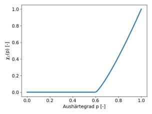
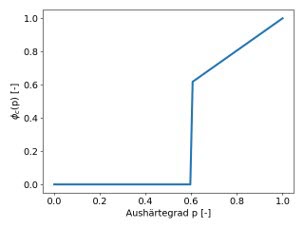
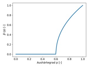
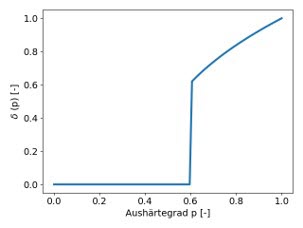
While the *MAT252 card does not support DoC-values on the history variables, it does support writing out four other history variables. If these are computed properly based on the DoC-values, they achieve the desired scaling of the material properties in the LS-DYNA application. The overall procedure is described below, while the corresponding commands are given in Output: Initial Stress Cards.
Read in the DoC-values stored as history variables at the integration points in the *INITIAL_STRESS_SOLID cards.
For every integration point, the four equations below and depicted in their respective figures are evaluated, where
 denotes the degree of cure. Furthermore,
  refers to a gel point above which the solidification of the
material begins. Both and the remaining five parameters (
refers to a gel point above which the solidification of the
material begins. Both and the remaining five parameters ( ,
,  ,
,  ,
,  , and
, and  ) are set for achieving the required characteristic
curves.
) are set for achieving the required characteristic
curves.For every element, write out *INITIAL_STRESS_SOLID cards containing the new history variables (
 ,
,  ,
,  , and
, and  ) at the integration points.
The following table contains the visualization of the curves given in their equations,
using these parameters:  ,
,  ,
,  ,
,  ,
,  , and
, and  .
.


For considering the DoC for the *MAT252 model, another option is to scale the material parameters directly within the Envyo application. As a result, a series of material cards is created and written out to the Envyo application's output file. In order to avoid writing out a modified material card for every element, in this approach, a clustering of elements is conducted, where each cluster represents a unique part with its own material. Otherwise, the strategy is almost equivalent to the one discussed in Output: Initial Stress Cards with the difference that here, each element has its own material definition instead of each integration point. The overall procedure is described below, and see Output: New *PART and *MAT252 Cards for the corresponding commands:
Read in the DoC-values stored as history variables at the integration points in the *INITIAL_STRESS_SOLID cards.
Compute the average DoC for each element.
Based on their average DoC values, sort the elements into buckets, which are characterized by their lower and upper DoC values. You must set the number of buckets and the ranges these cover.
For every bucket, create a new *PART card and corresponding *MAT252 card. The material properties for the given part are modified based on the average DoC associated with bucket limits. To achieve this, the functions in Output: Initial Stress Cards are evaluated first. Then, the resulting values are used according the seven equations below, where the parameters on the left-hand side are parameters for the new, modified *MAT252 card, while the values on the right-hand side with the ref extension refer to the parameters of the reference *MAT252, which is modified depending on the DoC. All elements that fall into a given bucket are added to that part.

(4–5)

(4–6)

(4–7)

(4–8)

(4–9)

(4–10)

(4–11)
For more information about these parameters, see the LS-DYNA User's Guide.
The *MAT252 material model represents an adhesive material and as such, it is typically augmented by the *MAT_ADD_COHESIVE keyword. Since depending on the number of requested buckets, a large amount of new parts and material cards are created, and adding the *MAT_ADD_COHESIVE cards by hand can potentially be a tedious task. Thus, these cards are also generated by the Envyo application based on certain inputs.
The previous section describes workflows that apply to the case, where instead of mapping the results from a source to a target mesh, only the data on a source mesh is modified. No actual mapping takes place. If the discussed workflows are used while transferring data from one mesh to another, the notions from Output: Initial Stress Cards and Output: New *PART and *MAT252 Cards are modified as follows: In both cases, after performing step 1, the DoC-data stored on the integration points is mapped from the source mesh to the target mesh. After that, the procedure continues from step 2 for the target mesh, and the Envyo application's input file must contain the appropriate commands regarding the mapping.
Below is a review of the commands regarding the *MAT252 keyword. First, the commands are covered which are the same for both workflows. Then, in Output: Initial Stress Cards and Output: New *PART and *MAT252 Cards, the additional commands are discussed which are specific to the workflows of Output: Initial Stress Cards and Output: New *PART and *MAT252 Cards, respectively.
| TargetMaterialModel = INT | This must be set to 252. |
| MAT252Parameter = DOUBLE, DOUBLE, DOUBLE, DOUBLE, DOUBLE, DOUBLE | This command is used to inform the Envyo application about the six
parameters that are necessary for computing the four functions given in
Output: Initial Stress Cards section. The six
parameters must be given in the following order: , , , , , and . |
| MAT252Strategy = INT |
1 - Output: Initial Stress Cards is triggered. 2 - Output: New *PART and *MAT252 Cards is triggered. |
| MAT252Definition = FILE | This command expects a .k- or .key-file containing a single instance of a *MAT252 keyword. The parsed keyword tells the Envyo application what material parameters to work with in this workflow. |
| DegreeOfCureHistoryPosition = INT | This command is used for telling the Envyo application at which history position is the DoC stored in the source mesh. |
If MAT252Strategy=1 is used, the above given commands must be extended by one additional command defined below.
| MAT252IHIS = INT | Typically, MAT252IHIS = 6 is recommended. |
If MAT252Strategy = 2 is used, a clustering pipeline is invoked as described in Output: New *PART and *MAT252 Cards. Below, the additional commands are listed and explained, which are mandatory for MAT252Strategy = 2.
| NumberOfBuckets = INT | Number of buckets for clustering the elements. If every bucket contains at least one element, the number of newly created parts equals NumberOfBuckets. Otherwise, *PART cards with no elements are deleted from the input deck. |
| StartingPartID = INT | Starting ID for the new parts resulting from the clustering of the elements. |
| SecID = INT | Each newly created *PART keyword requires the definition of a material ID and a section ID. While the material IDs are assigned to the parts by Envyo, you must define the section IDs. Currently, the section ID provided in this command is assigned to every new part. |
| StartingMatID = INT | Starting ID for the new *MAT252 keywords. |
| AddMatCohesiveParameters = DOUBLE, DOUBLE, DOUBLE, DOUBLE | Adhesive materials, such as the *MAT252 model, are often used in conjunction with the *MAT_ADD_COHESIVE keyword, which is characterized by the following five parameters: PID, ROFLG, INTFAIL, THICK, UNIAX. The pard ID (PID) for the newly created parts is already generated via the Envyo application. The remaining four parameters are parsed from this command and use for all *MAT_ADD_COHESIVE keywords. |
| MAT252ClusteringDegreeOfCureStartValue = INT | In addition to the number of buckets, you are required to provide a starting value for the DoC-range which is divided into buckets. In the current implementation start value of the range is by the command MAT252_Clustering_DegreeOfCureStartValue and the end value is DoC=1.0. Typically, the value pgel is used for this command, from which the solidification starts. However, if it is known a priori that all DoC value fall into range starting from much higher than pgel, other values can be used as well. Note that in all cases, an additional bucket is created that contains all elements in the DoC-range from 0.0 to start value set by you. |