


(Part A) Set up and process a simulation that can make use of the intra- and inter-particle collision statistics modules that are included by default in Rocky, and import a custom convex particle shape.
(Part B): Use custom Polyhedron (Envelope) User Process shape to define the spray zone, and then make use of the Residence Time information from that area to calculate the Coefficient of Variability (CoV). Analyze the collision statistics and contacts data that was collected.
The main purpose of this tutorial is to learn how to set up and process a simulation that can make use of the intra and inter-particle collision statistics modules that are included in Rocky.
We will be analyzing the simulation results and data collected in Part B and C.
The scenario considered is that of analyzing the performance of a tablet coating operation, which is often used in the pharmaceutical and food processing industries.
You will learn how to:
Import a custom particle shape
Use Original Size Scale to define particle size
Turn on the collection of various particle and contacts data
And you will use these features:
Modules, including:
Inter-particle Collision Statistics
Intra-particle Collision Statistics
Custom Polyhedron Import
Important: This ADVANCED tutorial contains fewer details, screenshots, and procedures than other Rocky tutorials.
An ADVANCED tutorial is designed for users who are more familiar with the Rocky user interface (UI), and already have a good understanding of the common setup and post-processing tasks.
If you do not already have this level of familiarity, it is recommended that you complete at least Tutorials 01 - 05 before beginning this one.

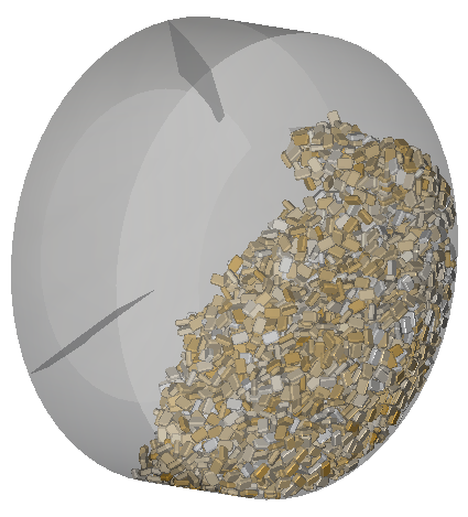
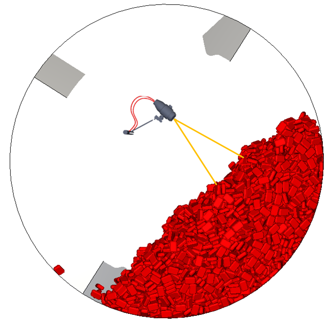
The primary geometry used in this tutorial is the Drum, shown above.
Also, two additional geometries will be used, including:
Spray_cone (used to create the polyhedron envelope)
Tablet (used to create the custom particle shape)
To get started with this tutorial, do the following:
Download the
dem_tut09_files.zipfile here .Unzip
dem_tut09_files.zipto your working directory.Open Rocky 2025 R2.
Create a new project.
Save the empty project to a location of your choosing.
Use the information in the table below to start setting up your Rocky project.
Tip: If you run into settings or procedures in these tables that you are not yet familiar with, please refer to the Rocky User Manual and/or other Tutorials (via the Introductory Tutorials and Advanced Tutorials) to find the detailed instructions you need.
Step Data Entity Editors Location Parameter or Action Settings A Study Study Study Name Coater B Physics Physics | Momentum
Numerical Softening Factor 0.01 [ - ]
For the Modules step, we will be turning on the collection of some additional data for particles, including:
Inter-particle Collision Statistics | Normal Impact Velocity:
Collects the mean, standard deviation, skewness, and kurtosis values of the impact relative velocity in the normal directions, resulting from the collisions recorded for each particle, during an output timestep.
Intra-particle Collision Statistics | Frequency:
Collects the collision frequency values measured by different regions of the representative particle of the selected particle set. This can be useful for analyzing collision incidence on the particle surface.
Use the information in the table that follows to define your modules and other project settings.
| Step | Data Entity | Editors Location | Parameter or Action | Settings |
|---|---|---|---|---|
| A | Modules | Modules | Inter-Particle Collision Statistics | (Enabled) |
| Intra-Particle Collision Statistics | (Enabled) | |||
| B | Modules ﹂Inter-Particle Collision Statistics | Inter-Particle Collision Statistics | Normal Impact Velocity | (Enabled) |
| C | Modules ﹂Intra-Particle Collision Statistics | Intra-Particle Collision Statistics | Frequency | (Enabled) |
| D | Geometries | Import Wall | Drum.stl with "m" for Import Unit | |
| E | Motion Frames | Create Motion Frame | ||
| F | Motion Frames ﹂Frame <01> | Frame | Name | Rotation Motion |
| Add Motion | ||||
| Start Time | 1 [s] | |||
| Type | Rotation | |||
| Initial Angular Velocity | 0, 0, 12 [rev/min] | |||
| G | Geometries ﹂Drum | Wall | Motion Frame | Rotation Motion⯆ |
| H | Materials ﹂Default Particles | Material | Use Bulk Density | (Cleared) |
| Density | 1150 [kg/m3] | |||
| I | Materials | Materials Interactions | Default Particles⯆ Default Boundary⯆ | Static Friction | 0.39 [ - ] |
| Dynamic Friction | 0.39 [ - ] | |||
| Restitution Coefficient | 0.78 [ - ] | |||
| Materials Interactions | Default Particles⯆ Default Particles⯆ | Static Friction | 0.45 [ - ] | ||
| Dynamic Friction | 0.45 [ - ] | |||
| Restitution Coefficient | 0.78 [ - ] | |||
| J | Particles | Create Particle | ||
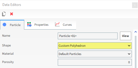
For the Particles step, we will create a custom polyhedron particle set by importing an .stl file of a tablet shape, as explained on the next section.
Select the new <Particle <01> entry, and then from the main Particle tab, define the Shape as Custom Polyhedron.
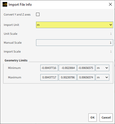
From the Select file to import dialog, navigate to the dem_tut09_files folder that you previously downloaded, find the geometry folder, select the Tablet.stl file, and then click Open.
From the Import File Info dialog, ensure Import Unit is defined as m, and then click OK.
Note: The tablet shape we just imported is a perfect convex. To learn how Rocky handles importing convex shapes that are not perfect, refer to the Appendix section at the end of this tutorial.
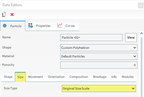
For this tutorial, because we are importing our own custom shape, we will be using Original Size Scale for the Size Type.
The Original Size Scale method allows you to use the size of the imported particle geometry as the base from which you can scale your final particle size.
For example:
A Scale Factor of 1 is equal to the original imported size (100%).
A Scale Factor or 0.5 is equal to half the original size (50%).
A Scale Factor of 2 is equal to double the original size (200%).
To set the particle size, do the following:
From the Size sub-tab, select Original Size Scale from the Size Type list.
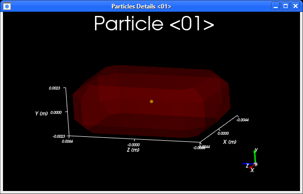
To visualize the newly created particle, click the View button. A new Particles Details window will appear showing the (transparent) particle geometry, its geometric center (yellow dot), and its center of mass (blue dot).
From the Coloring tab, enable the Edges checkbox to see the meshing in the Particle Details view.
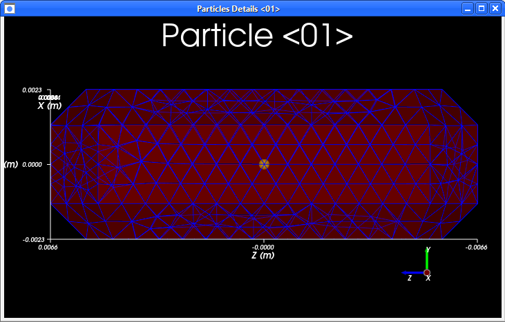
Tip: To ensure a good analysis of properties distribution on the particle surface, ensure that you use a particle with a high resolution of triangles next to the edges.
Use the information in the table that follows to continue setting up your project.
Step Data Entity Editors Location Parameter or Action Settings A Inlets and Outlets Create Volumetric Inlet B Inputs ﹂Volumetric Inlet <01>
Volumetric Inlet | Particles Add row (x1) (1) Particle | Mass
Particle <01> @ 2.7 [kg] Volumetric Region | Region Seed Coordinates 0, -0.1, 0 [m] Geometries | Drum (Enabled) Use Geometries to Compute (Enabled)
A Contact in Rocky refers to a specific location on a geometry or particle that has experienced a collision with another particle during the simulation.
Always during processing, Rocky calculates and makes use of Contacts data. But to save file space, you can choose whether or not to keep it.
For this tutorial, we will enable the collection of the Contacts data so that we can analyze the Stress Components of the particles later in post-processing.
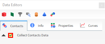
From the Data panel, select Contacts and then from the Data Editors panel, ensure the Contacts tab is selected.
Enable the Collect Contacts Data checkbox.
Now, use the information in the table that follows to define your Solver parameters.
Step Data Entity Editors Location Parameter or Action Settings A Solver Solver | Time Simulation Duration 60 [s] Solver | General Simulation Target GPU⯆
Note: Because this tutorial has convex particles, processing with GPU will be faster if you have that option.
With a 3D View window opened, your Data panel and Workspace should look similar to the below image.
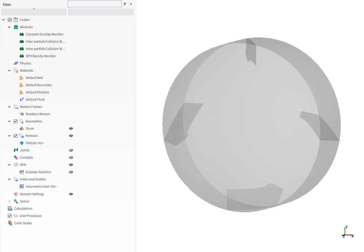
From the Solver entity, click Start.
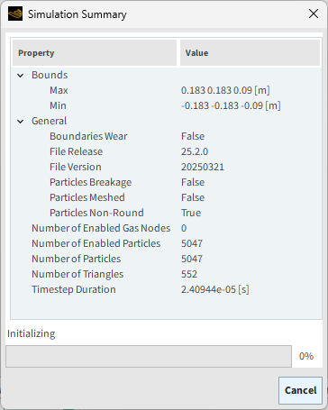
The Simulation Summary screen appears, then processing begins.
Tip: You can use the Auto Refresh checkbox to view in a 3D View window the results during processing.
This completes Part A of this tutorial, in which Rocky was used to set up and process a tablet coating simulation.
During this tutorial, it was possible to:
Turn on the collection of particle collision statistics and contacts data for later analysis.
Import a custom particle shape.
Use Original Size Scale to define particle size.
What's Next?
If you have completed this tutorial successfully, then you are ready to move on to Part B and post-process this project.
The tablet shape we imported in this tutorial is a perfect convex, meaning it contains no faces that form dents or hollows.
Rocky categorizes even mostly convex shapes as concave if there is even the smallest dent or hollow detected.
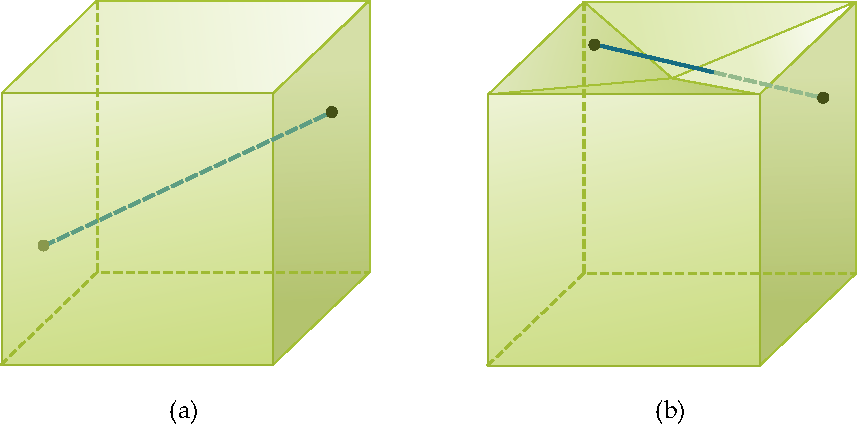
In a convex shape, any straight line that connects any two faces will always be contained inside the shape (a).
In a concave shape, a similar line connecting two faces may have portions that fall outside the shape (b).
Because Rocky uses different calculations for shapes it categorizes as concave, it is very important that you make sure Rocky categorizes your shape the way you want.
If you ever want to import a particle shape that is not a perfect convex (but you still want Rocky to treat it as such), you can take one of the following steps:
Improve your convex .stl design and then re-import it into Rocky.
-OR-
Allow Rocky to redraw the shape to ensure it is categorized as convex.
If Rocky detects that your convex shape is imperfect, it will ask you to choose one of the following options (as shown):
Keep the shape as is: The particle will be treated as concave, and will use concave-based calculations.
Convert the shape to convex: Rocky will redraw the imperfect shape to ensure it is categorized as convex, and will use convex-based calculations.
The main purpose of this tutorial is to analyze the results and data that was collected from the tablet coating simulation we set up and processed in Part A.
You will learn how to:
Import a custom Polyhedron User Process shape
Use the Residence Time information to calculate the Coefficient of Variability (CoV)
Analyze the collision statistics and contacts data that was collected
And you will use these features:
Polyhedron (envelope) User Process
Particles Calculations (Residence Time)
Eulerian Statistics
Time Statistics properties
Important: This ADVANCED tutorial contains fewer details, screenshots, and procedures than other Rocky tutorials.
An ADVANCED tutorial is designed for users who are more familiar with the Rocky user interface (UI), and already have a good understanding of the common setup and post-processing tasks.
If you do not already have this level of familiarity, it is recommended that you complete at least Tutorials 01 - 05 before beginning this one.
If you completed Part A of this tutorial, ensure that Rocky project is open. (Part B will continue from where Part A left off.)
If you did not complete Part A, do all of the following:
Download the
dem_tut09_files.zipfile here .Unzip
dem_tut09_files.zipto your working directory.Open Rocky 2025 R2. (Look for Rocky 2025 R2 in the Program Menu or use the desktop shortcut.)
Important: To make use of the Rocky project file provided, you must have Rocky 2025 R2 or later. If you have an earlier version of Rocky, please upgrade Rocky to the latest version, or complete Part A from scratch.
From the Rocky program, click the Open Project button, find the dem_tut09_files folder, then from the tutorial_09_A_pre-processing folder, open the tutorial_09_A_pre-processing.rocky file.
Process the simulation. (From the Data panel, select Solver and then from the Data Editors panel, click the Start button.)
With the processing complete, we can now begin analyzing the simulation results.
With coating processes like the one shown, it is really important to guarantee that each Particle spends enough time in the coating region (spray zone).
Rocky allows the creation of a new Property variable, Residence Time, which computes the time each particle spent inside a predefined User Process region (Cube, Cylinder, or Polyhedron).
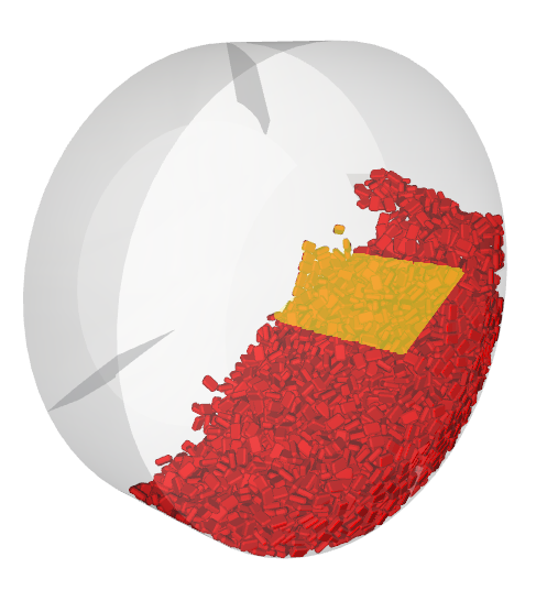
For this tutorial, two Polyhedron User Processes, representing two elliptic spray cones, will be imported using an .stl geometry.
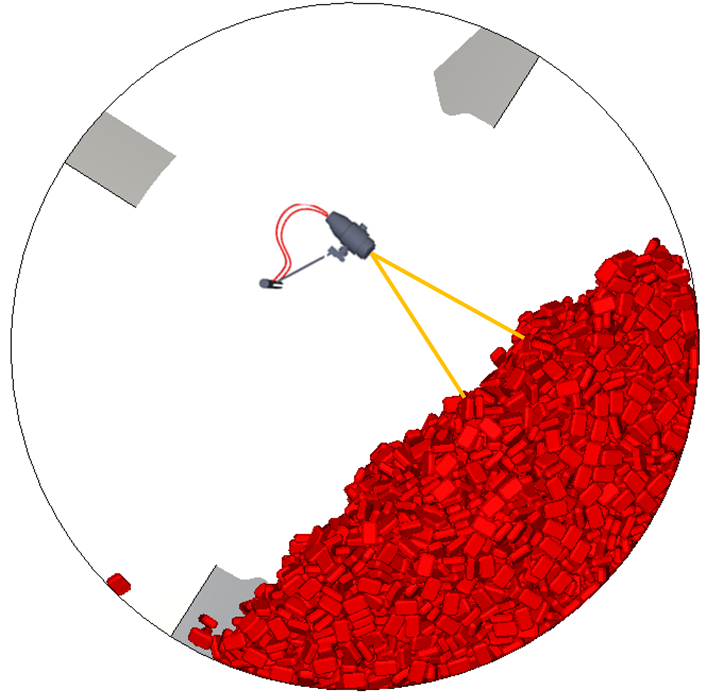
Representation of the Tablet Coating Process with Nozzles and Spray Cone:
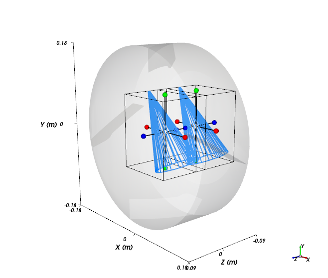
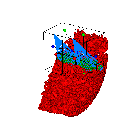
Drum Showing Newly Imported Polyhedron User Process Shape:
To import the first Polyhedron:
From the Data panel, right-click Particles, point to Processes, and then select Polyhedron (Envelope).
From the Select the STL file for the polyhedron dialog, navigate to the dem_tut09_files folder that you previously downloaded, find the geometry folder and then select the Spray_Cone.stl file, and then click Open.
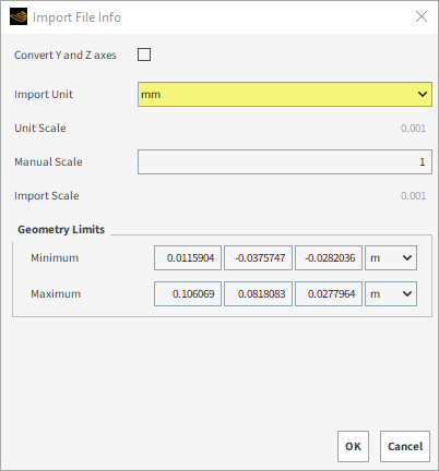
From the Import File Info dialog, set the Import Unit to mm, and then click OK.
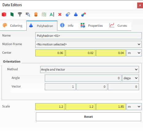
From the Data panel, under User Processes, select the newly created Polyhedron <01> entry.
From the Data Editors panel, on the Polyhedron tab, set the Center and the Scale.
To import the second Polyhedron:
Repeat the process on the previous section to create another Polyhedron (Envelope) User Process, select the same Spray_Cone.stl geometry, and import it in mm.
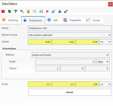
From the Data panel, under User Processes, select this new Polyhedron <02> entry and then from the Data Editors panel, set the Center and the Scale.
Note: In this version of Ansys Rocky you are able to duplicate Polyhedron User Processes.
After this second import you should have two Polyhedrons representing the spray nozzles.
Now that we have imported the two cones, we can apply the Residence Time Particle Calculation over them to analyze how much time each Particle spends inside each of the cone regions.
From the Data panel, right-click Particles, point to Particles Calculations, point to Residence Time, and then select Polyhedron <01> (as shown). A new Calculations entity named Residence Time (Polyhedron <01>) will be created.
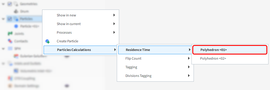
Repeat this step for the Polyhedron <02> User Process.
From the Data panel, select Residence Time (Polyhedron <01>), and then set Stop Time to 60s.
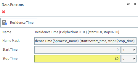
Repeat this step for Residence Time (Polyhedron <02>).
By combining the Residence Time results from each cone, we will be able to see how well the full spray zone is coating the particles over time.
We will do this combination by creating a Custom Property for Particles.
Use the information in the table that follows to continue setting up your project.
Step Item Location Parameter or Action Settings A Particles Properties Add new custom property (button) B Add new (dialog box) Name Total Residence Time Output unit s Inputs | Residence Time (Polyhedron <01>) (Enabled) Inputs | Residence Time (Polyhedron <02>) (Enabled) C Custom Property (dialog box) Expression A+B
A new property called Total Residence Time (Custom) will appear among the Particles Properties.
This can be used like any other Property to color the Particles and/or create new plots.
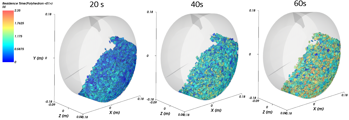
From the Data Editors panel for the main Particles entity, select the Coloring tab and then under Nodes, select Total Residence Time (Custom) for Property.
Use the Time slider to view the changes at different output times.
Note: You may have to hide the Polyhedrons user processes using the eye icons on the Data panel.
As shown in the screenshots below, some particles spend more time in the spray zone than others. At 60 s, the coating is still rather uneven as seen by the presence of many different colored particles.
The Inter-tablet Coefficient of Variability (CoV) can be defined as the ratio between the Standard Deviation of coating mass over the Average of coating mass.
The coating mass depends primarily on the Residence Time inside the spray zone, so we can define the CoV as:

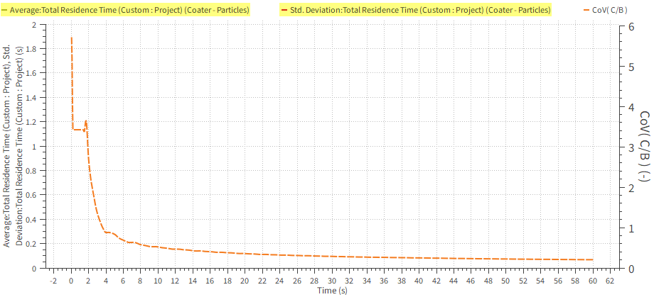
To create the CoV analysis, we need to start with a Time Plot. Follow the instructions on the next few slides.
Create a new Time Plot. (From the Window menu, click New Time Plot (Ctrl+T).)
Use the information in the table that follows to define the Time Plot.
| Step | Item | Location | Parameter or Action | Settings |
|---|---|---|---|---|
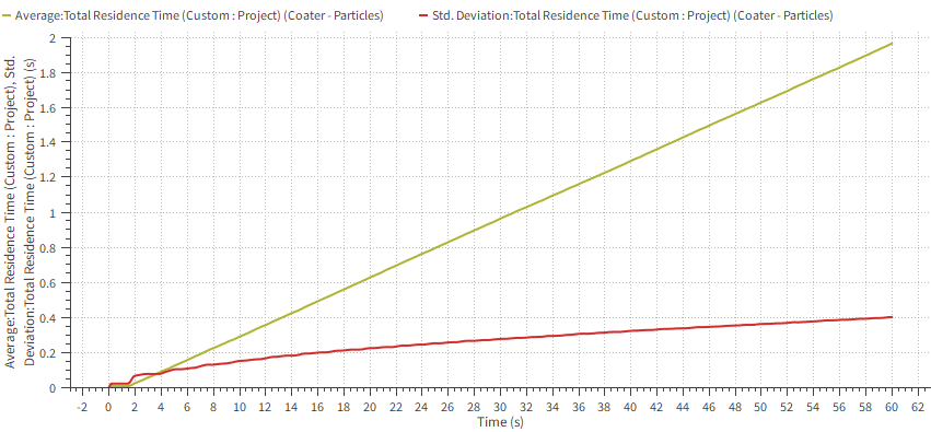
| A | Particles | Properties | Total Residence Time (Custom) | Drag and drop onto the Time Plot window | |
| B | Select the Statistics to Plot (dialog box) | Average | (Enabled) | |
| Std. Deviation | (Enabled) | |||
Right-click whithin the plot grid, point to Axes Layout, and then click By Quantity.
Now, let's calculate the Coefficient of Variability (CoV) by creating a new Formula in the Time Plot.
Use the information in the table that follows to define the formula.
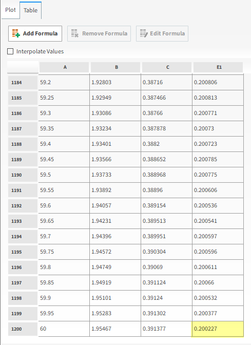
Step Item Location Parameter or Action Settings A Time Plot Table (tab) Add Formula B Add Expression (dialog box) Curve Caption CoV Curve Expression B/C Note: For the formula to work, the expression must represent the Std. Deviation divided by the Average of the Total Residence Time (Custom) property. If your columns appear in a different order, adjust the formula accordingly.
Scroll down to the end of the table and note that the CoV at 60 s reaches only 20%.
Switch back to the Plot tab.
At the top of the tab, click the curve names for Std. Deviation and then Average to hide them from the plot (as shown). The CoV curve will be the only one visible.
From the Plot tab, right-click the Time axis, and then click Customize Axis.
Use the information in the table below to define the Axis Configuration values.
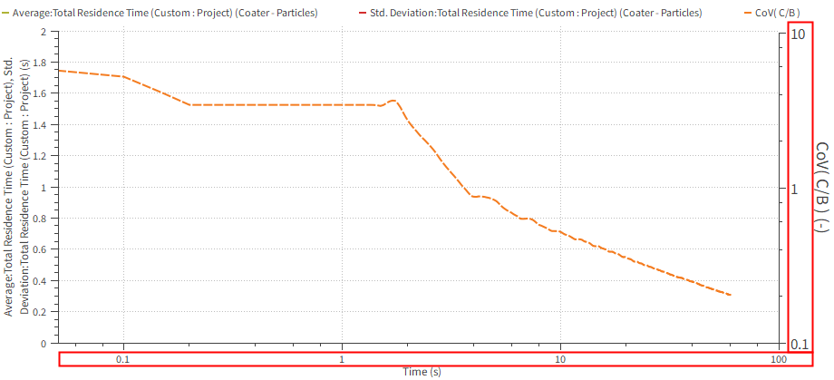
Step Item Location Parameter or Action Settings A Axis Configuration (dialog box) Axis | Time (s) Values | Limits User Defined Values | Min 0.05 [s] Values | Max 100 [s] Values | Step 1 [s] Scale Options | Logarithmic Scale (Enabled) Axis | CoV( B/C ) ( - )
Values | Limits User Defined Values | Min 0.1 [s] Values | Max 10 [s] Values | Step 1 [s] Scale Options | Logarithmic Scale (Enabled) Click OK.
When you configure the graph with the CoV results in a log-log plot (right and bottom axes only), you obtain the graph shown.
A common analysis is to extrapolate the CoV results to estimate the time needed for a specific value of CoV.
With the extrapolation, you do not need to run the full, extended simulation (which can take many, many hours to process).
The linear region at the end of the log-log plot (steady state) is seen after 10 s of simulation time, and will be used as the basis for the extrapolation.
It is possible to extrapolate the CoV results by using a separate spreadsheet program.
We will accomplish this by exporting the data out of the plot into a .csv file, opening that file in a separate spreadsheet program, and then using that program to manipulate the data as needed.
Let's start by exporting the Curve data:
Right-click an empty space within the plot, point to Export, and then click Curves.
From the Export Configuration dialog, clear the Average and Std. Deviation checkboxes (as shown), and then click OK.
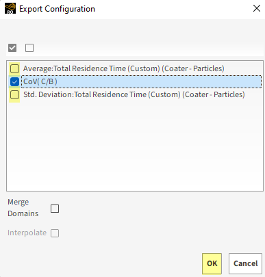
From the Export Curve(s) dialog, enter a File Name for the resulting .csv file, choose a folder location, and then click Save.
Open the resulting .csv file in a spreadsheet program.
Using the spreadsheet program, fit a curve to the CoV results by using the following equation:

(9–1)
where:
 is the CoV
  and
and  are fitting constants
  is the time
For the extrapolation, use the steady state time range between 10 - 60 s. (Results shown as orange dotted line.)
Using a desired regularization limit of 6.25% CoV (shown as green dotted line), locate the time it meets the fitted CoV (shown as red dot).
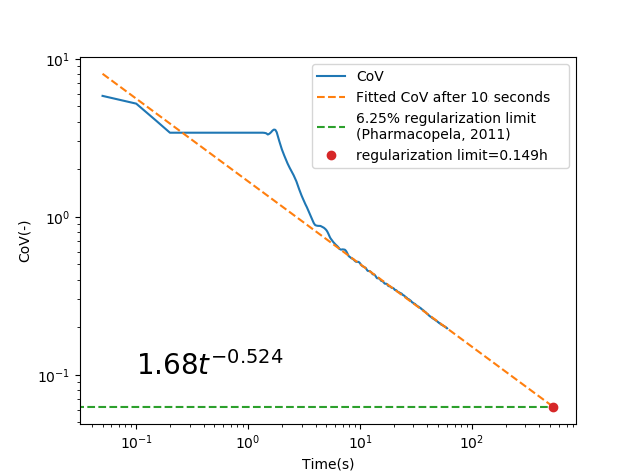
According to the literature (Boehling et al., 2016 [1]), the value of the exponential constant should be close to -0.5.
Based on the graph on the previous slide, the following conclusions can be made:
The adjusted value obtained by the Rocky CoV results achieved a value of -0.524, which is close to the desired value.
To reach the desired 6.25% CoV regulation limit, you need approximately 0.149 hours (or 536.4 seconds) of simulation time.
The discrete Properties can be converted into continuous values, by averaging the values over discretized regions, using the Eulerian Statistics User Process.
The Eulerian Statistics should be created on a Cube or Cylinder User Process.
For this case, a Cylinder will be created.
Use the table below to define these processes.
Step Data Entity Editors Location Parameter or Action Settings A Particles Create a Cylinder User Process B User Processes ﹂Cylinder <01>
Cylinder Size 0.365, 0.2, 0.365 [m] Center 0, 0, 0 [m] … | Orientation Method Angles⯆ Rotation 90, 0, 0 [dega] C User Processes ﹂Cylinder <01>
Create a Eulerian Statistics User Process D User Processes ﹂Eulerian Statistics <01>
Eulerian Statistics Radial Divisions 20 [ - ] Tangential Divisions 72 [ - ] Axial Divisions 1 [ - ]
This will discretize the Cylinder into 72 circular sectors, each one having 20 divisions in the radial direction. A single bin is defined in the axial direction.
New Properties specifically for Eulerian Statistics will be available to plot on the Eulerian's bins, including Stress Components, Transformed Velocity, and so on.
Once the Eulerian Statistics is created, the Transparency, Edges, and Color can be modified on the Coloring tab:
With a 3D View opened, use the information in the table that follows to define these values.
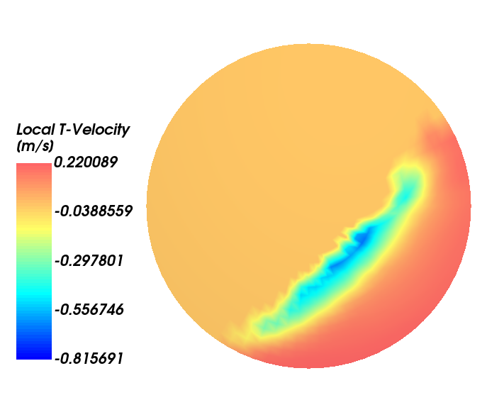
Step Data Entity Editors Location Parameter or Action Settings A User Processes ﹂Eulerian Statistics <01>
Coloring Faces | Property Local T-Velocity⯆ Faces | Show on Node? (Enabled) Edges (Cleared) Tip: When you enable a Property for Faces, the option Show on Node? allows for the continuous display of the plotted Property.
Tip: Ensure the Visible checkbox is enabled.
From the Data panel, click the Particles eye icon to hide the previous particle calculation.
Updated results shown.
Rocky can also create Time Statistics of those Properties, providing Average, Maximum, Minimum, and Sum values.
To evaluate the maximum shear stress during the bed cycles, do the following:
From the Data Editors panel, select the Properties tab for the Eulerian Statistics.
From the top right of the selected tab, click the icon for Add and edit time statistics properties (as shown).
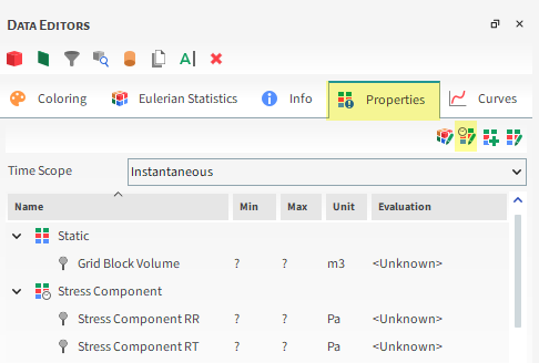
From the Edit time statistics properties dialog, click the Add button (green plus).
From the Add time statistics properties window, specify the Start and Stop time of the analysis, the Operations and the Properties to evaluate (as shown), and then click OK.
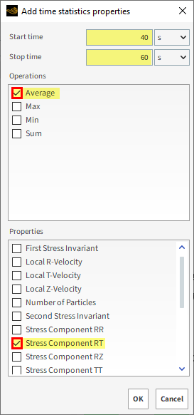
Click OK again on the Edit time statistics properties window.
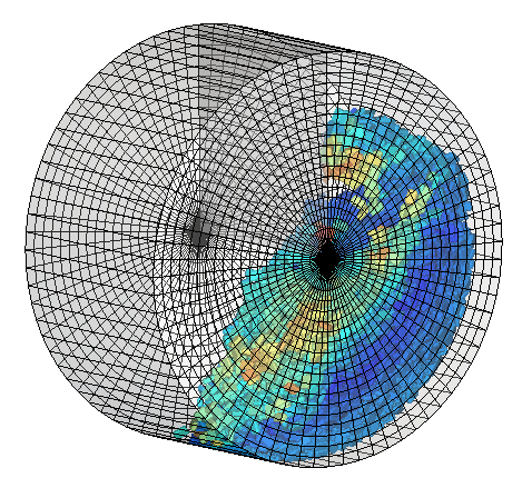
From the Properties tab, under Time Analysis, select the newly created Average of Stress Component [40 s, 60 s] property, and then drag and drop it onto the 3D View for Eulerian Statistics. (Results shown below.)
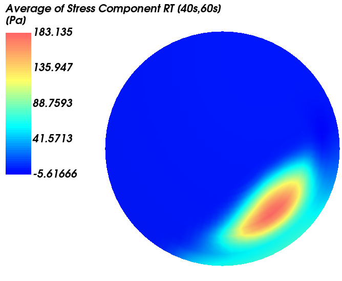
This average analysis helps identify the location in the coater where particles experience a higher value of Stress.
Important: To be able to analyze Stress Components, you must have enabled the Collect Contacts Data checkbox from Contacts entity on the Data panel prior to processing your simulation.
As a reminder, we took this step in Part A, so this data should now be available to analyze.
Earlier in the setup portion of this tutorial (Part A), you turned on the collection of Intra-particle Collision Statistics.
The intra-particle collision statistics represent the full transient analysis of all particles in the domain shown on a single representative particle.
During the simulation, relevant collision data is stored between two consecutive output time levels.
It is important to note that each result represents the time average between the current output and the previous.
So, if you want to do an analysis spanning the full simulation time, you need to include a new expression to account for all of the outputs.
Another important point is the geometry resolution of the particle. To achieve a good analysis, ensure that you use a particle with a high resolution of triangles next to the edges.
Use the information in the table below to create this new particle time statistics property.
Step Data Entity Editors Location Parameter or Action Settings A Particles ﹂Particles <01>
Properties Add and edit time statistics properties (button) B Edit time statistics properties (dialog box) Add property (button) C Add time statistics properties (dialog box) Start time 40 [s] Stop time 60 [s] Operations | Average (Enabled) Properties | Frequency (Enabled) From the Data panel, under Particles, select Particle <01>.
From the Data Editors panel, on the Particle tab, click View.
A new Particles Details window opens.
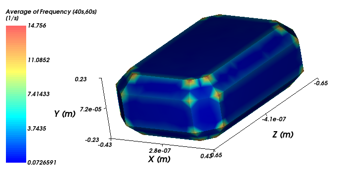
From the Properties tab, under Time Analysis, select the newly created Average of Frequency [40s, 60s] property, and then drag and drop it onto the Particles Details window. (Results shown below.)
From the Particle <01> entity, on the Coloring tab, clear the Transparency checkbox.
This shows the average collision frequency per particle recorded in different regions (triangles) of the particle shape.
We can see that the number of collisions is highest at the corners and edges and lowest on the flat surfaces of the particle.
We can therefore conclude that when particles of this shape collide with other particles and with the drum walls, they do so most often on their corners and edges.
Earlier in the setup portion of the tutorial (Part A), we turned on the collection of Inter-particle Collision Statistics.
These can be useful when you need to extract data considering all collisions that happened to a certain particle during an interval between two consecutive output times.
For example, with impact velocity, you could relate that data to the chances of the particle breaking or causing it to de-agglomerate. With duration, you could relate that data to a certain mass or heat transfer process, or to a certain chemical reaction.
It is important to note that each result represents the time average of data collected during an interval between two consecutive output times.
On the next slides, the Impact Velocity will be analyzed to show potential moments of high energies (and possible breaking).
From the Data panel, select Particles.
From the Data Editors panel, select the Properties tab.
Under Translational Velocity, right-click Velocity : Impact : Normal : Mean, point to 3D View, and then click Show in new 3D View. (Results shown.)
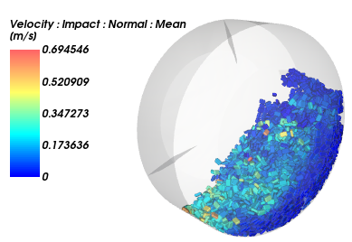
Tip: To see the particles, you may need to make the Drum geometry transparent.
This completes Part B of this tutorial, in which Rocky was used to post-process a Tablet Coating simulation.
During this tutorial, it was possible to:
Import two custom polyhedron user process shapes to analyze residence time.
Calculate, plot, and then extrapolate the Coefficient of Variability (CoV).
Analyze the Intra- and Inter-particle collision statistics data that was collected.
Use Eulerian Statistics and Time Statistics to evaluate Stress Components.
What's Next?
If you completed this tutorial successfully, then you are ready to move on to Part C and further analyze the spray zone.
The purpose of this tutorial is to use the Coating Visibility Wizard on the tablet coating simulation we set up and processed in Part A to further investigate the coating variability on the particles.
This method uses the camera position of a 3D View window to define the spray area. The wizard then computes the amount of exposure on each particle (or particle region), which is a more accurate method than the procedure we used in Part B.
You will learn how to:
Import and run saved PrePost scripts in the PrePost Scripts panel
Use the wizard results to analyze the Coefficient of Variability (CoV)
Use the wizard results to analyze the visibility on the particle shape itself
And you will use these features:
PrePost Scripts panel
Important: This ADVANCED tutorial contains fewer details, screenshots, and procedures than other Rocky tutorials.
An ADVANCED tutorial is designed for users who are more familiar with the Rocky user interface (UI), and already have a good understanding of the common setup and post-processing tasks.
If you do not already have this level of familiarity, it is recommended that you complete at least Tutorials 01- 05 before beginning this one.
If you completed Part A (and/or Part B) of this tutorial, ensure that Rocky project is open. (Part C will continue from where Part A and/or Part B left off.)
If you did not complete Part A (nor Part B), then do all of the following:
Download the
dem_tut09_files.zipfile here .Unzip
dem_tut09_files.zipto your working directory.Open Rocky 2025 R2.
Important: To make use of the Rocky project file provided, you must have Rocky 2025 R2 or later. If you have an earlier version of Rocky, please upgrade Rocky to the latest version, or complete Part A from scratch.
From the Rocky program, click the Open Project button, find the dem_tut09_files folder, then from the tutorial_09_A_pre-processing folder, open the tutorial_09_A_pre-processing.rocky file.
Process the simulation. (From the Data panel, select Solver and then from the Data Editors panel, click the Start button.)
With the processing complete, we can now begin analyzing the simulation results.
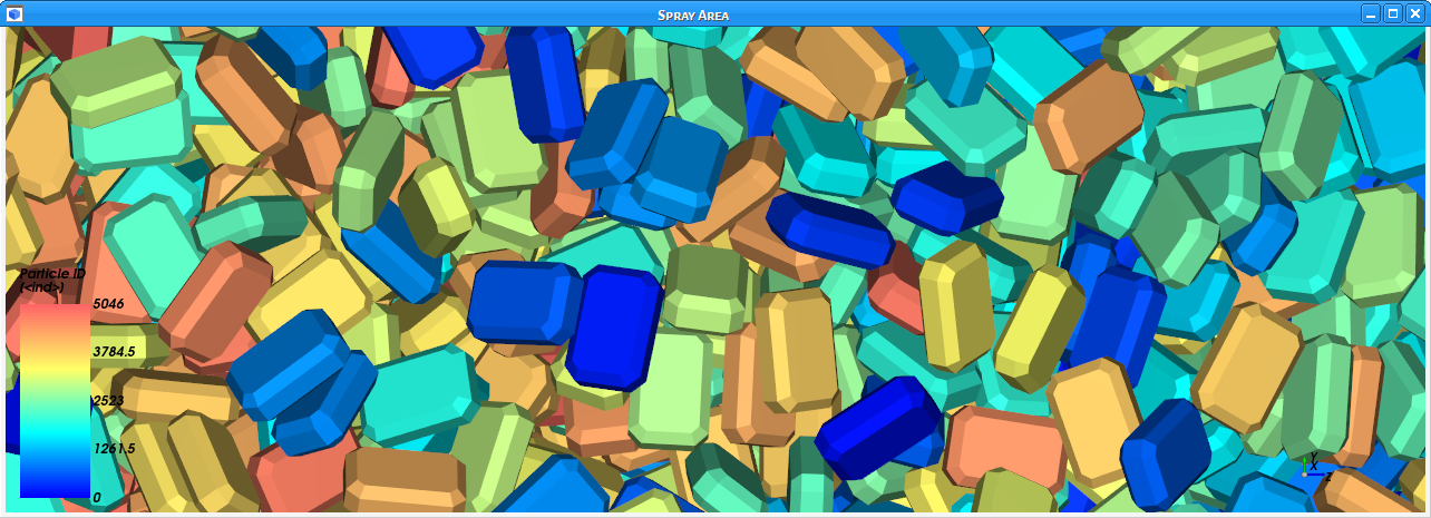
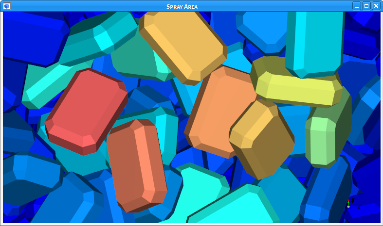
The spray area of the coating operation will be determined by the camera location, orientation, and level of zoom of a 3D View window.
The window's focus will act like a nozzle and the visible particles will be exposed to the coating.
Representation of the tablet coating process with nozzles and spray region:
Region of interest (in yellow) where the 3D View window should be focused:
The Visibility is the Percentage that a particle (or particle region) occupies within the camera view in a given time and is accounted by a pixel by pixel verification.
Particles Visibility (camera view)
Particles Visibility (another angle)
The visibility computation is available only through the Coating Visibility Wizard.
The Coating Visibility Wizard is a complete application that runs inside Rocky and enables you to quickly and easily define the nozzle parameters for your coating applications.
Preview capabilities are available inside the wizard, which enables to visualize the Spray Mask and Nozzle parameters before running the wizard.
The wizard includes embedded post-processing capabilities, which enables you to analyze the coating Visibility results.
This wizard calculates the coating Visibility for each output time and then automatically creates new properties based on those calculations.
To start, show the PrePost Scripts panel by selecting it from the Tools menu.
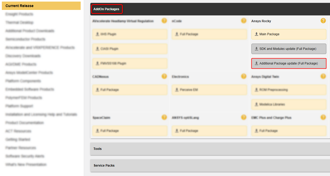
To download the Coating Visibility Wizard, click here. Click Current Release and make sure the selected Release matches the Rocky version you have.
Navigate to AddOn Packages, and then from the Ansys Rocky tab download the Additional Package.
Extract the Rocky Additional Package zip folder to your computer. Open the Coating Visibility Wizard folder and extract the coating_visibility_wizard.zip folder to your computer.
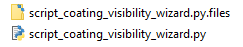
From the coating_visibility_wizard folder, copy both the script_coating_visibility_wizard.py script and the script_coating_visibility_wizard.py.files folder to your clipboard.
From the Rocky PrePost Scripts panel, with the first Scripts shared across projects tab selected, click the Open Scripts Directory button.
Within the %HOMEPATH%\Documents\Rocky\Scripts folder that opens, paste the script and folder you copied.
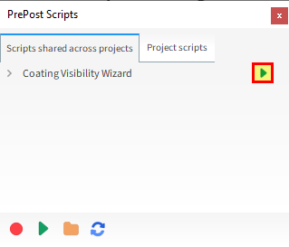
The new script will appear in the PrePost Scripts panel on the Scripts shared across projects tab.
To run the Coating Visibility Wizard, do the following:
Click the Playback Script button.
Note: The wizard calculates the visibility at each separate output. Because of that, it might take some time to complete the calculations.
Because the Coating Visibility Wizard is a complete application that runs inside Rocky, you can not interact with Rocky while the wizard is running.
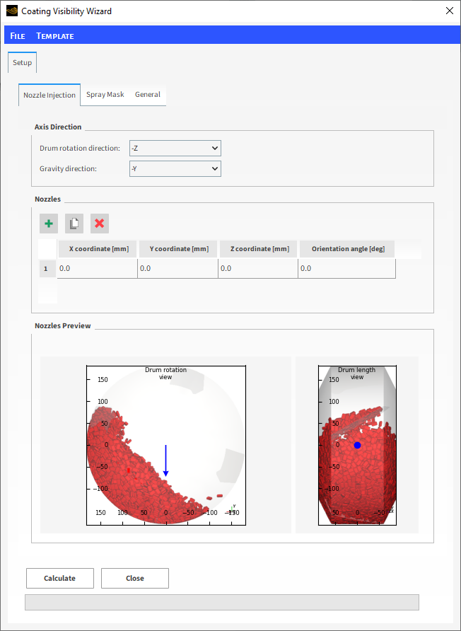
The Coating Visibility Wizard will appear as a new window showing the Setup tab.
This wizard enables you to easily define the nozzles parameters. You can add as many nozzles as you need and then configure them.
Note: When more than one nozzle is used, the wizard will change the camera position at each output time in order to analyze the region of each nozzle.
Follow the procedures below to define your setup (as shown).
On the Nozzle Injection sub-tab, from the Axis Direction field, define the Drum rotation direction as +Z.
From the Nozzles field, click the Add button (green plus) to create an nozzle entry.
For both 1 and 2 nozzles, define the Y coordinate, Z coordinate and Orientation angle.
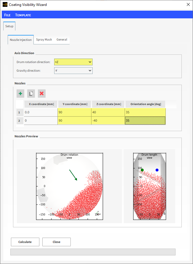
Note: The options for the Axis Direction will be used to position the nozzles. Ensure you define it correctly and check it on the Nozzles Preview field.
This wizard supports masks for the visibility calculation in case you want to calculate the visibility in rectangular, elliptical and custom areas.
The mask emulates the spray shape of the nozzle.
Select the Spray Mask sub-tab, and then define all of the following (as shown):
Spray mask type
White core horizontal length
White core vertical length
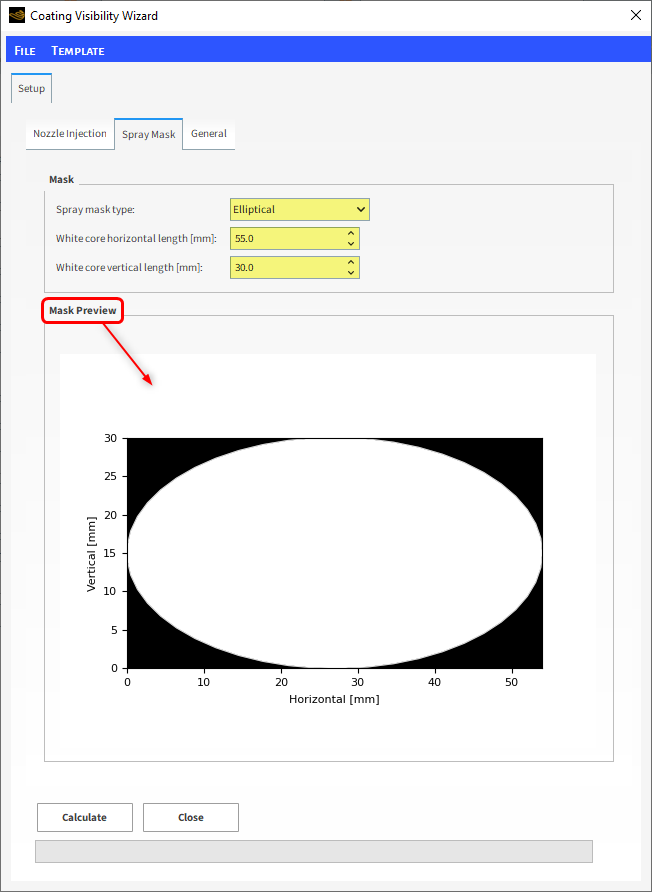
Note: The Mask Preview will help you to correctly define the mask (as shown).
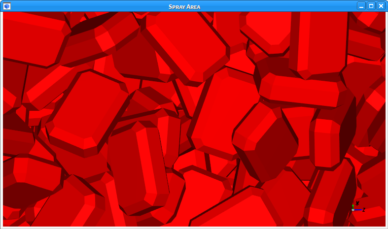
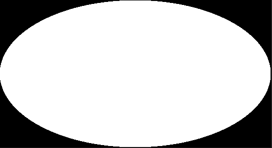
The darker the pixel, the higher the opacity. Thus, the black borders of the image will be ignored by the camera. The images below illustrate how the visibility is computed combining the camera view and the mask:
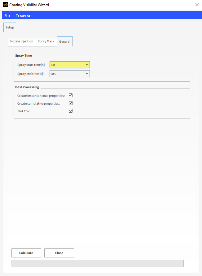
On the General sub-tab, you can define options for the Spray Time and Post Processing.
Follow the procedures below to continue defining your wizard setup.
Select the General sub-tab, define the Spray start time as 3.0 (as shown) and check the other options to match the screenshot.
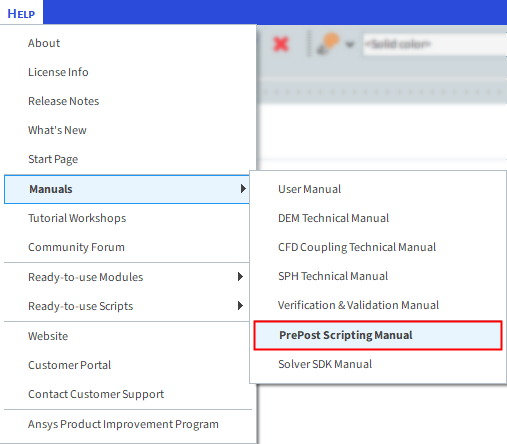
For more information about this wizard and its parameters, access the Scripts Manual from the Help menu tab (as shown).
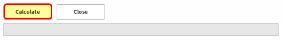
Now your Coating Visibility Wizard is set up. From the Setup tab, click the Calculate button:
Note: The wizard calculates the visibility at each separate output. Because of that, it might take some time to complete the calculations.
After the wizard finishes its calculations, a confirmation message will appear (as shown).
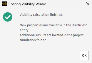
Note: You can remain inside the wizard to do some types of visibility post-processing (as shown on the next sections). Outside of the wizard, you also have new properties for the Particles entity in Rocky and new files located in the project's simulation folder.
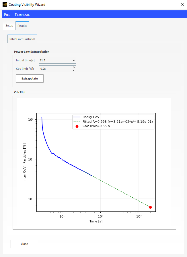
After the wizard finishes its calculations, the wizard will point to a new Results tab.
This wizard automatically generates an analysis of Inter-tablet coating variability (CoV). It also generates an extrapolation for the available data.
You can easily find the amount of time related to a specific CoV value.
In addition, the wizard also gives you the option to change the extrapolation parameters. From the Results tab, in the Power Law Extrapolation section, you have the following options (as shown):
Initial time (used to define the beginning of the interpolation range)
CoV limit
To generate the CoV plot of the previous side, firstly the wizard need to estimate the coating mass one particle receives in a given output interval:
 | (9–2) |
where:
 is the coating mass of the
  -th particle, when time is equal to
  .
. is the spray mass flow rate.
  is the particles visibility of the -th particle, when time is equal to .
  is the output interval.
To estimate the total coating mass:
 | (9–3) |
where:
 is the cumulative visibility of the -th particle, when time is equal to .
The Inter-tablet coating variability ( ) can be defined as the ratio between the Standard
Deviation of coating mass over the Average of
coating mass in a given time.
) can be defined as the ratio between the Standard
Deviation of coating mass over the Average of
coating mass in a given time.
 | (9–4) |
It can be rewritten as:
 | (9–5) |
The product  is constant, so:
 | (9–6) |
Therefore, it is possible to calculate the through the ratio between the Standard
Deviation of Total Cumulative Visibility over
the Average of Total Cumulative
Visibility.
 | (9–7) |
The Coating Visibility Wizard shows the CoV results in a log-log plot (vertical and horizontal scales shown).
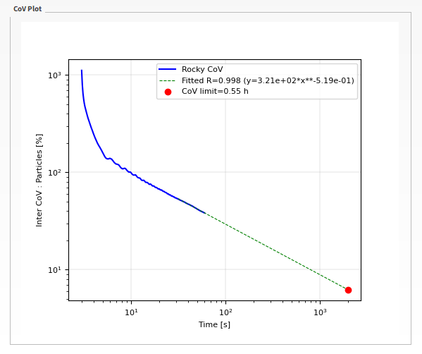
A common analysis is to extrapolate the CoV results to be able to estimate the time needed for a specific value of CoV.
With the extrapolation, you do not need to run the full, extended simulation (which can take many, many hours to process).
The wizard itself defines the linear region, which is at the end of the log-log plot (steady state) after 30 s of simulation time, and was used as the basis for the extrapolation.
The linear region can be fitted by a power law equation:
 | (9–8) |
where:
 is the CoV.
  and
and  are fitting constants.
  is the time.
According to the literature (Boehling et al., 2016 [1]), the value of the exponential constant should be close to -0.5.
Based on the graph on the previous slide, the following conclusions can be made:
The adjusted value obtained by the Coating Visibility Wizard's CoV results achieved a value of -0.486, which is close to the desired value.
To reach the desired 6.25% CoV regulation limit, you need approximately 0.7 hours (or 2520 seconds) of simulation time, which is much longer than the simulation time estimated earlier in Part B of this tutorial.
After finishing the analyses inside the Coating Visibility Wizard, you can close the wizard and go back to the Rocky UI.
The wizard has created two new particles properties for each nozzle:
Note: You will also have these properties for each particle group in case you have a shaped particle. In this case, these properties are related to each triangle of the particle surface.
Instantaneous Visibility: Returns the fraction of the 3D View area exposed per particle at the currently selected output time. If a faceted particle is used, this returns the average triangle visibility at the current output for all the particles in each Particle Group.
Cumulative Visibility: Returns the cumulative visibility from the initial output time up to the currently selected one. If a faceted particle is used, this returns the cumulative triangle visibility from the initial output time up to the currently selected output time for all the particles in each Particle Group.
Also, for each of the previously properties, the wizard has created a new property to evaluate the contribution of each nozzle. The following equation was applied for each property:
 | (9–9) |
where:
 is the total visibility property for the coater.
  is the visibility property of each nozzle.
The wizard has created two new particles properties for the total visibility:
Note: You will also have these properties for each particle group in case you have a shaped particle. In this case, these properties are related to each triangle of the particle surface.
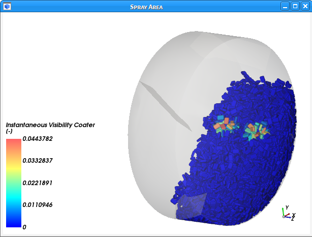
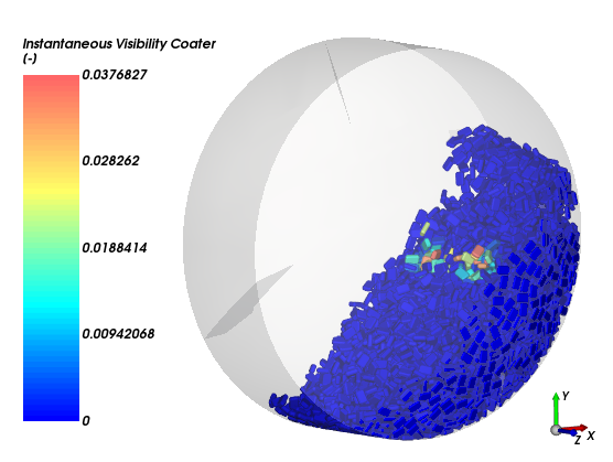
Instantaneous Visibility Coater
Cumulative Visibility Coater
To access the Particles Visibility property:
From the Data panel, select Particles.
From the Data Editors panel, select the Properties tab.
To visualize the Particles Visibility, drag and drop Instantaneous Visibility Coater onto a 3D View window (results shown).
To visualize the Cumulative Visibility:
From the Data panel, select Particles.
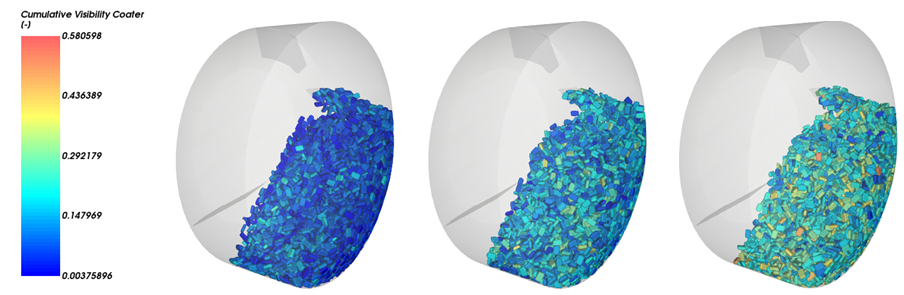
From the Data Editors panel, select the Properties tab, and then drag and drop Cumulative Visibility Coater onto a 3D View window. (Results shown.)
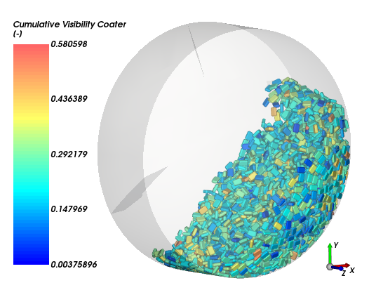
For this tutorial, we are mainly interested in the Cumulative Visibility, which is directly proportional to the injected mass.
Note: Use the Time slider to see how the property changes over time.
As shown in the screenshots below, some particles spend more time in the spray zone than others. At 60 s, the coating is still rather uneven as seen by the presence of different colored particles.
To visualize the Cumulative Visibility on the Particle Group:
From the Data panel under Particles, select Particle <01>.
From the Data Editors panel, on the main Particle tab, click the View button. A new Particles Details window appears.
From the Data Editors panel, select the Properties tab, and then drag and drop Cumulative Visibility Coater onto the Particles Details window.
From the Time toolbar, select the last output time.
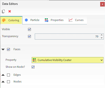
From the Coloring tab, clear the Transparency checkbox (results shown).
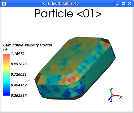
From the Data Editors panel, on the Coloring tab, under Faces, enable the Show on Node? checkbox (as shown).
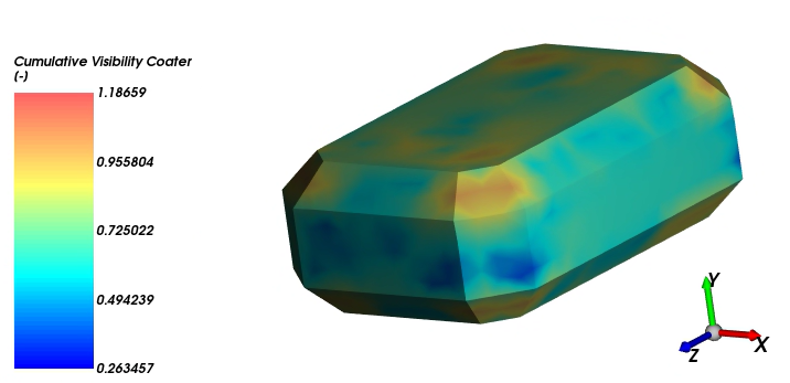
The results show that at 60 seconds into the simulation, most parts of the particle achieved some amount of coating coverage, with the highest values concentrated on the corners as well as the the upper and lower flat regions of the particle.
This completes Part C of this tutorial, in which Rocky was used to analyze the spray zone and particle coating results from the Tablet Coating simulation we set up and processed in Part A.
During this tutorial, it was possible to:
Import and run the Coating Visibility Wizard.
Analyze the CoV results generated by Coating Visibility Wizard, and the particle visibility itself.
What's Next?
If you completed this tutorial successfully, then you are ready to move on to next tutorial.