


(Part A) Define the mantle and shaft movements required for a Cone Crusher, set up Tavares breakage parameters, and collect Boundary Collision Statistics for later post-processing.
(Part B) Track the position of tagged particles, compute the resulting PSD of resulting fragments, isolate broken fragments from whole particles, and calculate the average power draw.
The two main purposes of this tutorial are to learn how to define the mantle and shaft movements required for a Cone Crusher simulation, and how to set up Tavares breakage model parameters.
You will learn how to:
Turn on the collection of intensities data for later post-processing of power draw
Define mantle and shaft movements for a cone crusher simulation
Turn on random particle orientation
Set up Tavares breakage model parameters
And you will use these features:
Boundary Collision Statistics Module
Cone Crusher Motion Frame
Particle Orientation
Tavares Particle Breakage
Important: This ADVANCED tutorial contains fewer details, screenshots, and procedures than other Rocky tutorials.
An ADVANCED tutorial is designed for users who are more familiar with the Rocky user interface (UI), and already have a good understanding of the common setup and post-processing tasks.
If you do not already have this level of familiarity, it is recommended that you complete at least Tutorials 01- 05 before beginning this one.
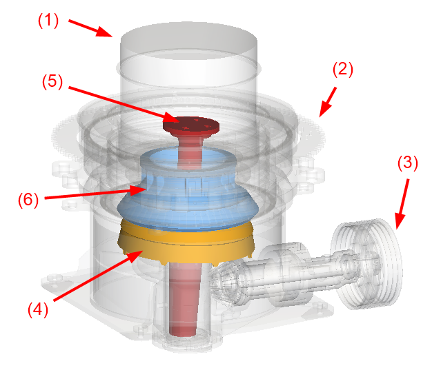
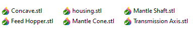
The geometries in this tutorial are composed of:
(1) Feed Hopper (Choke Feed)
(2) Housing
(3) Transmission Axis
(4) Mantle Cone
(5) Mantle Shaft
(6) Concave
The .stl files can be found in the tutorial directory.
To get started with this tutorial, do the following:
Download the
dem_tut08_files.zipfile here .Unzip
dem_tut08_files.zipto your working directory.Open Rocky 2025 R2.
Create a new project.
Save the empty project to a location of your choosing.
For this tutorial, information about Power on the boundary will be used.
Therefore, we must enable the collection of Boundary Collision Statistics during the Modules step.
Use the information in the table that follows to start setting up your Rocky project.
Tip: If you run into settings or procedures in these tables that you are not yet familiar with, please refer to the Rocky User Manual and/or other Tutorials (via the Introductory Tutorials and Advanced Tutorials) to find the detailed instructions you need.
Step Entity Editors Location Parameter or Action Settings A Study 01 Study Study Name Cone Crusher B Modules Modules Boundary Collision Statistics (Enabled) C Modules ﹂Boundary Collision Statistics
Boundary Collision Statistics Intensities (Enabled)
Note: With Intensities enabled, Rocky will collect the average dissipation and impact power values measured by each individual geometry triangle.
For the Geometries step, we will import the following six separate geometry files in .stl format, disable the Feed Hopper geometry during initial particle release, and then add a surface (to associate with an inlet) to release particles into the domain.
Use the information in the table that follows to continue setting up your Rocky project.
Step Data Entity Editors Location Parameter or Action Settings A Geometries Import Wall All six .stl geometry files with "mm" for Import Unit B Geometries ﹂Feed Hopper
Wall Enable Time 3 [s] C Geometries Create a Circular Surface D Geometries ﹂Circular Surface <01>
Circular Surface Center Coordinate 0, 1.65, 0 [m] Max Radius 0.46 [m]
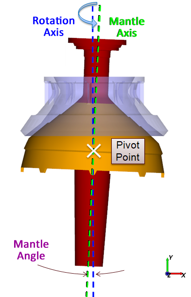
In this tutorial, we will be creating cone crusher movements, which are defined by the following motions:
The Mantle rotates eccentrically around the vertical axis, pressing the particles on the Concave and promoting breakage. At the same time, it is free to rotate around the Shaft.
The intersection between the Mantle Axis and the Rotation Axis characterizes the Pivot Point.
It is important to have your mantle geometry rotated by the desired Mantle Angle and to know in which direction this is done to properly set up the Cone Crusher movement.
These motions can be created in Rocky with a special Cone Crusher Frame that is added during the Motion Frames step.
When the new Cone Crusher Frame is added to your project, the following options are available in the Data Editors panel:
Pivot Point: Coordinate of the point around which the Mantle and Shaft will pivot.
Rotation Axis: The axis around which the Mantle and Shaft are rotated.
Rotational Velocity: The angular velocity along the Rotation Axis.
Initial Orientation: The vector about which the Mantle and Shaft begin their rotation.
Start/Stop Time: Time in which the motion starts and stops.
In addition, the Cone Crusher Frame will automatically create two separate motions that are designed to be applied to the appropriate geometries.
Important: These motions appear only in the Motion Frame list for the imported Geometry and are not listed under Motion Frames in the Data panel.
These two motions include the following:
Cone Crusher <01> (Mantle) for the Mantle Cone geometry.
Cone Crusher <01> (Shaft) for the Mantle Shaft geometry.
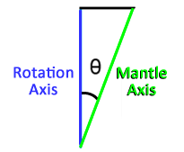
How to calculate Initial Orientation:


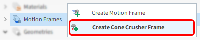
For the Motion Frames step, we will add a type of motion frame that is specific to the cone crusher:
From the Data panel, right-click Motion Frames, and then select Create Cone Crusher Frame.
Use the information in the table below to define the new frame.
Step Data Entity Editors Location Parameter or Action Settings A Motion Frames ﹂Cone Crusher <01>
Cone Crusher Frame Pivot Point 0, 0.687, 0 [m] Rotational Velocity 15.708 [rad/s] Initial Orientation 0.03943, 0.9992, 0 [m] Start Time 2.5 [s]
The frame's two components can now be assigned to their respective geometries.
Use the information in the table that follows to assign the new motions.
Step Data Entity Editors Location Parameter Location Settings A Geometries ﹂Mantle Cone
Wall Motion Frame Cone Crusher <01> (Mantle) B Geometries ﹂Mantle Shaft
Wall Motion Frame Cone Crusher <01> (Shaft)
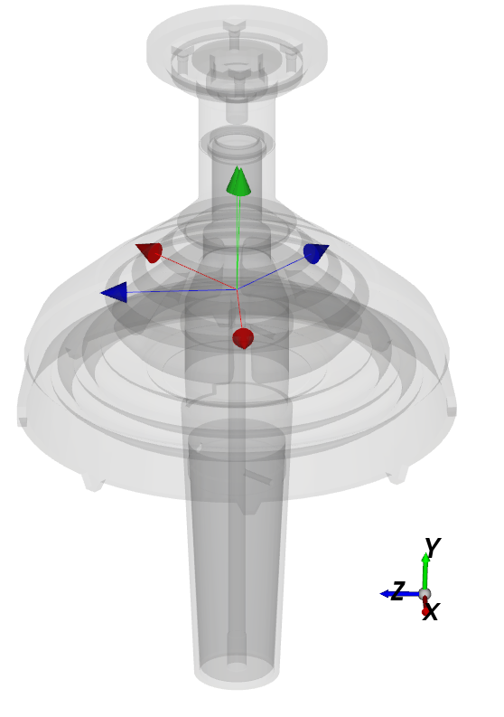
At this point, the movement can be previewed.
From the Data panel, click Motion Frames and then click Preview.
A new Motion Preview window will appear. To better see the results:
Use the Data panel eye icons to hide all the geometries except Mantle Cone and Mantle Shaft.
Also, to better see the two separate frame axes, enable the Transparency checkbox for both the Mantle Cone and Mantle Shaft geometries.
Note: When you play the preview, no motions will be seen before 2.5 s.
For the Materials step, two materials will be used:
One for all wall parts (Default Boundary), which we will use as defined by default.
Another for the particles (Default Particles), which we will modify.
Use the information in the table below to define these materials and their interactions.
Step Data Entity Editors Location Parameter or Action Settings A Materials ﹂Default Particles
Material Use Bulk Density (Cleared) Density 2500 [kg/m3] Young's Modulus 1e+07 [N/m2] B Materials Materials Interactions | Default Particles ⯆
Default Boundary ⯆
Static Friction 0.7 [s] Dynamic Friction 0.7 [s]
Important: The Young's Modulus value was lowered to speed up tutorial processing. For breakage simulations, it is recommended to set these values between 5e+08 and 1e+09 Pa.
For the Particles step, we will create a new (rock-like) polyhedron-shaped particle group, in a range of sizes, with random orientation, and with the Tavares breakage model enabled.
Use the information in the table below to start defining your particles.
Step Data Entity Editors Location Parameter or Action Settings A Particles Create Particle B Particles ﹂Particle <01>
Particle Shape Polyhedron Particle | Size Add size row (x3) (1) Size | Cumulative % 0.2 [m] @ 100 [%} (2) ... 0.15 [m] @ 70 [%] (3) ... 0.1 [m] @ 30 [%] (4) ... 0.08 [m] @ 10 [%]
For this tutorial, we will change the orientation of the particles as they are injected into the inlet.
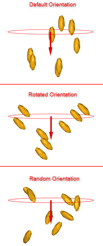
By default, particles are injected into the domain perpendicular to the inlet (top image).
You can change the orientation to have all particles come in at a defined angle (middle image), come in at random angles (bottom image), and many options in between.
For this tutorial, we will set a random orientation, as specified below.
To set the orientation of the particle:
From the Orientation sub-tab, enable the Random Angle checkbox, and then define the Half Range (x,y,z) values (as shown).
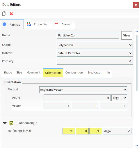
Tip:
For default particle shapes, or other symmetrical custom shapes, setting your values to 90, 90, 90 ensures a completely random orientation in all directions.
For non-symmetrical custom particle shapes (such as a bottle), you will need to set your values to 180, 180, 180 to ensure a completely random orientation.
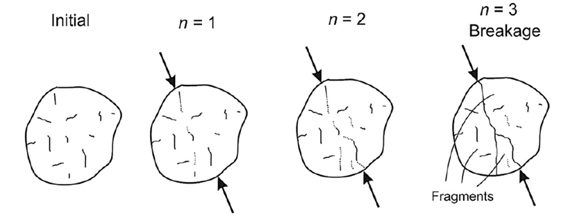
For this tutorial, we will enable the Tavares breakage model.
Like Ab-T10, the Tavares model is based upon the Voronoi fracture particle subdivision algorithm.
However, the breakage energy probability and resulting fragment size distribution are based upon the Tavares et al. (UFRJ) approach, which:
Models fractures by low-energy stressing, which is most relevant when particles are subject to a complex series of loading events, as within crushers.
Has been able to describe the progressive growth of crack-like damage that ultimately leads to the fracture of a particle under stresses significantly lower than those required for breakage in a first event.
Tip: Refer to the Tavares Breakage Model Description and Calibration Guidelines white paper for more information.
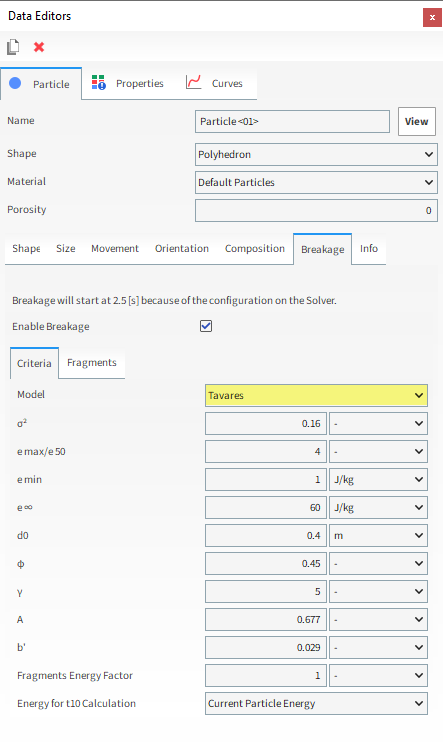
To set the Breakage Model:
From the Breakage sub-tab, select the Enable Breakage checkbox.
From the Breakage | Criteria tab, define the Model and leave all the model's parameters as default.
From the Breakage| Fragments sub-tab, define Minimum Absolute Size and Distribution model.
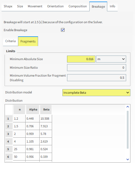
Important: The Minimum Absolute Size value used in this tutorial was increased to speed up processing time. Refer to the Fragment size distribution models section of the DEM Technical Manual for details on how best to set this value.
For the Inlets and Outlets step, we will create a Particle Inlet and then set our Circular Surface as the location from which we want particles to enter the simulation.
For the Solver step, we will also define our breakage start and delay times.
Use the information in the table below to finish setting up your project.
Step Data Entity Editors Location Parameter or Action Settings A Inlets and Outlets Create Particle Inlet B Inputs ﹂Particle Inlet <01>
Particle Inlet Entry Point Circular Surface <01>⯆ Particle Inlet | Particles
Add row (x1) (1) Particle | Mass Flow Rate Particle <01>⯆ @ 350 [t/h] … | Time Stop 3 [s] C Solver Solver | Time Simulation Duration 12 [s] Breakage | Start 2.5 [s] … | Delay After Release 1 [s] Solver | General Simulation Target CPU ⯆
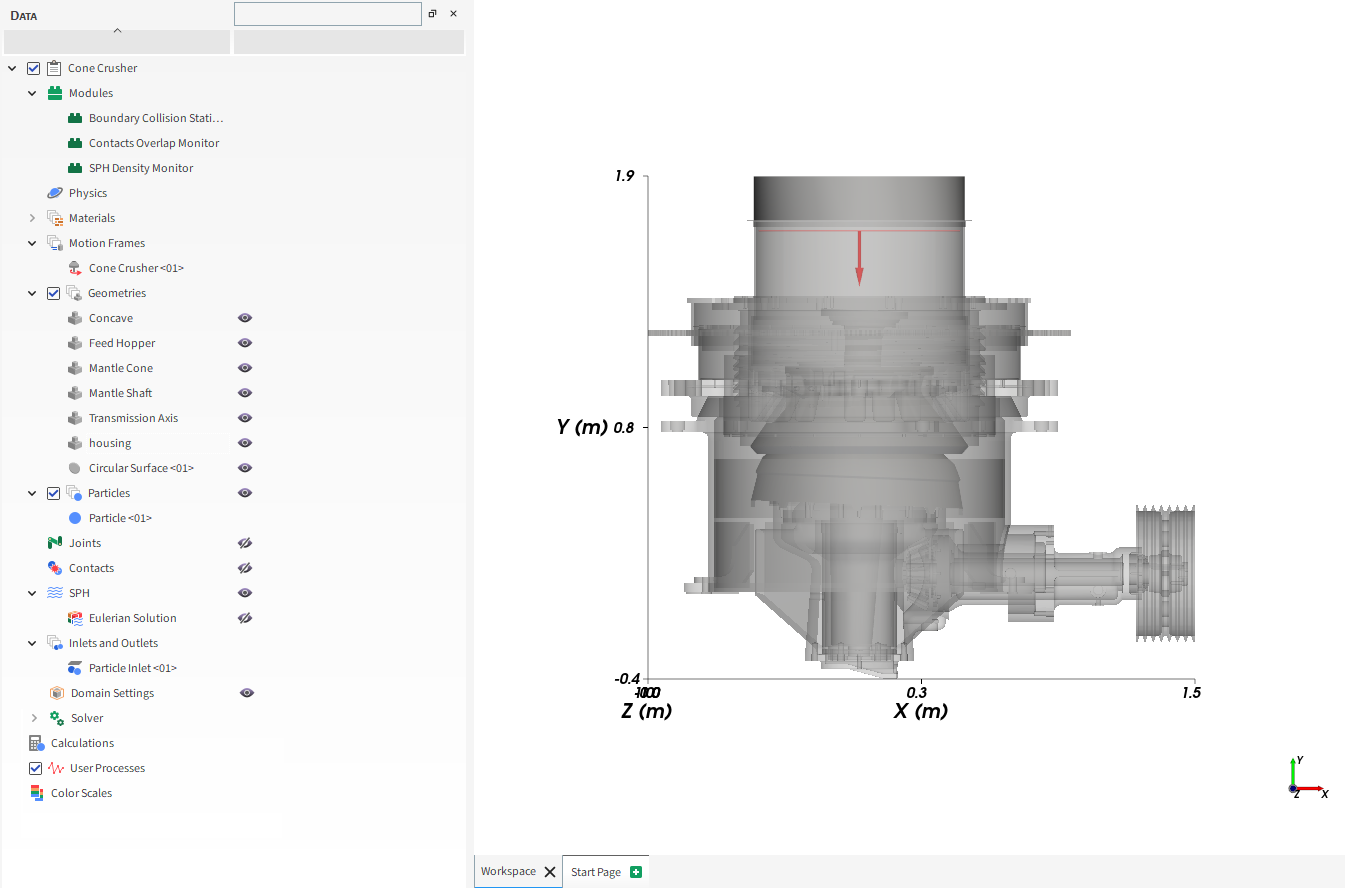
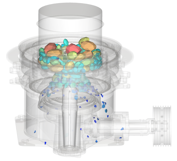
With a 3D View window opened, your Data panel and Workspace should look similar to the image below.
From the Solver entity, click Start.
The Simulation Summary screen appears (as shown), then processing begins.
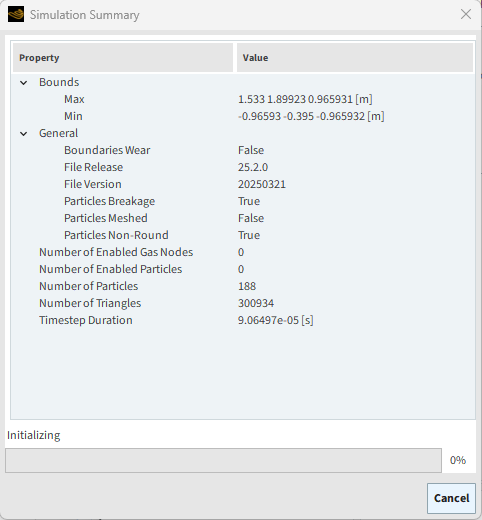
Tip: You can use the Auto Refresh checkbox to view in a 3D View window the results during processing.
This completes Part A of this tutorial, in which Rocky was used to set up and process a cone crusher simulation.
During this tutorial, it was possible to:
Collect Boundary Collision Statistics data for later post-processing of power draw.
Use the specialized Cone Crusher Frame to easily set up and apply specific mantle and shaft motions.
Set particles to be released in a random orientation.
Enable the simulation of Breakage phenomena using the Tavares model.
What's Next?
If you completed this tutorial successfully, then you are ready to move on to Part B and post-process this project.
The main purpose of this tutorial is to learn how to analyze the results from the Cone Crusher simulation that we set up and processed in Part A.
You will learn how to:
Track the position of tagged particles
Compute the PSD of the resulting fragments
Isolate the broken fragments from the whole particles
Calculate the Average Power Draw
And you will use these features:
Histograms
Time Plots
User Processes, including:
Cylinder
Cube
Particles Time Selection
Property
Particle Calculations, including:
Divisions Tagging
Important: This ADVANCED tutorial contains fewer details, screenshots, and procedures than other Rocky tutorials.
An ADVANCED tutorial is designed for users who are more familiar with the Rocky user interface (UI), and already have a good understanding of the common setup and post-processing tasks.
If you do not already have this level of familiarity, it is recommended that you complete at least Tutorials 01- 05 before beginning this one.
If you completed Part A of this tutorial, ensure that Rocky project is open. (Part B will continue from where Part A left off.)
If you did not complete Part A, do all of the following:
Download the
dem_tut08_files.zipfile here .Unzip
dem_tut08_files.zipto your working directory.Open Rocky 2025 R2. (Look for Rocky 2025 R2 in the Program Menu or use the desktop shortcut.)
Important: To make use of the Rocky project file provided, you must have Rocky 2025 R2 or later. If you have an earlier version of Rocky, please upgrade Rocky to the latest version, or complete Part A from scratch.
From the Rocky program, click the Open Project button, find the tutorial_08_A_pre-processing folder, and then open the tutorial_08_A_pre-processing.rocky file.
Process the simulation. (From the Data panel, select Solver and then from the Data Editors panel, click the Start button.)
Once processing is complete, you can analyze the resulting Particle Size Distribution (PSD) of the fragments.
We will do this by:
Using a Cube User Process to define the area beneath the cone.
Applying a Particles Time Selection User Process to the Cube in order to capture data for the whole simulation length.
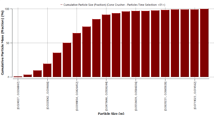
Plotting the resulting Particle Size data in a Histogram.
Use the information in the table below to set up the Cube and Particles Time Selection User Processes.
Step Data Entity Editors Location Parameter or Action Settings A Particles Create a Cube User Process B User Process ﹂Cube <01>
Cube Center 0, 0.08, 0 [m] Magnitude 1.4, 1.1, 1.4 [m] C User Processes ﹂Cube <01>
Create a Particles Time Selection User Process D User Processes ﹂Particles Time Selection <01>
Time Selection Domain Range All ⯆ Tip: If you run into settings or procedures in these tables that you are not yet familiar with, please refer to the Rocky User Manual and/or other Tutorials to find the detailed instructions you need.
Use the information in the table below to create and configure the Histogram.
Step Item Parameter or Action Settings A User Processes ﹂Particles Time Selection <01>
Show in new Histogram by Particle Size B Histogram (window) Configure histogram (button) C Configure Histogram (dialog box) Weight Particle Mass ⯆ Number of Bins 20 Cumulative Bins (Enabled) Percent Values (Enabled)
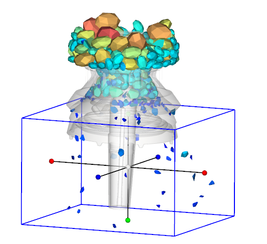
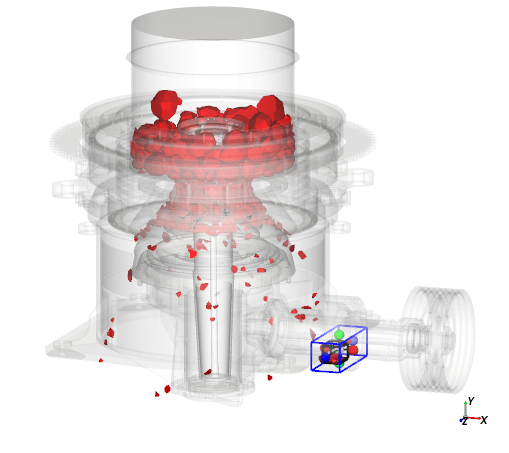
In the last Timestep of the simulation, you can observe that some Particles are accumulating in an open space of the transmission housing (in the Blue cube) (as shown).
Using the Divisions Tagging Calculation of the Particles in the hopper, we can identify from what section of the hopper these particles are coming from, which is helpful information for improving the equipment design.
For this case, we will create a Cylinder User Process at an Output Time far enough into the simulation that the Hopper is full of particles.
From the Time toolbar, select the [60] 3 s output time.
Use the information in the table below to create and configure the Cylinder.
Step Data Entity Editors Location Parameter or Action Settings A Particles Create a Cylinder User Process B User Processes ﹂Cylinder <01>
Cylinder Size 1.01, 1.01, 1.01 [m] Center 0, 1.2, 0 [m] With the Cylinder set up, right-click Particles, point to Particles Calculations, point to Divisions Tagging, and then click Cylinder <01>.
This will generate divisions within the cylinder that was selected, the result of which can be seen in a 3D View window.
From the Data panel, under Calculations, select the new Divisions Tagging (Cylinder <01>) entry.
Use the information in the table to define the Tagging values.
Step Data Entity Editors Location Parameter or Action Settings A Calculations ﹂Divisions Tagging (Cylinder <01>)...
Tagging Time Ranger Filter | Domain Range After Time Time Range Filter | Initial 3 [s] Tangential Divisions 12
Tip: With a 3D View window open and selected, you can visualize the tagged particles by enabling the Transparency checkbox from the Coloring tab.
Color Particles using the newly added Property:
From the Data panel, select Particles.
From the Data Editors panel, select the Coloring tab.
Under Nodes, change the Property to Divisions Tagging (Cylinder <01>)
Tip: Use the eye icons next to Cylinder and Cube (under User Processes in the Data panel) to hide the Cylinder and Cube coloring and show only the Particles coloring.
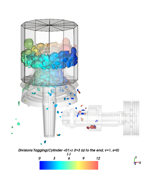
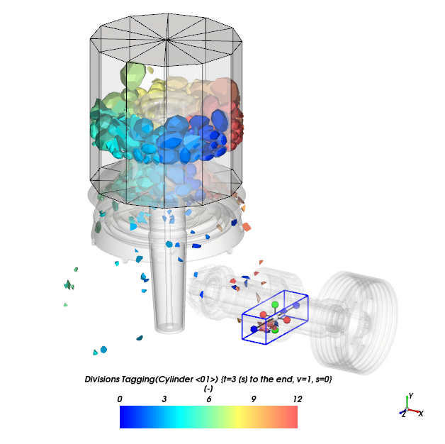
Display the final Output Time.
You should now see all of the following:
Hopper divided in 12 circular sectors.
Particles and Fragments colored by the division they started in.
The accumulated Fragments colored by their original position in the hopper.
Tip: You can duplicate a 3D view by pressing Ctrl +
D, selecting View > Window, or
right-clicking in the 3D view and choosing Duplicate.
Lastly for this analysis, a Cube will be added to separate the accumulated Fragments from the rest of the Particles.
Use the information in the table to define this new Cube.
Step Data Entity Editors Location Parameter or Action Settings A Particles Create a Cube User Process B User Processes ﹂Cube <02>
Cube Center 0.77, -0.017, 0 [m] Magnitude 0.24, 0.24, 0.54 [m]
Then, another Histogram will be created to show the hopper region from which the accumulated Fragments are originating.
Use the information in the table to define the Histogram.
Step Item Location Parameter or Action Settings A User Processes ﹂Cube <02>
Properties | Divisions Tagging (Cylinder <01>)...
Show in new Histogram B Histogram (window) Configure histogram (button) C Configure Histogram (dialog box) Number of Bins 12 Properties Divisions Tagging (Cylinder <01>)... Limits User Defined ⯆ Min 0.5 [-] Max 12.5 [-]
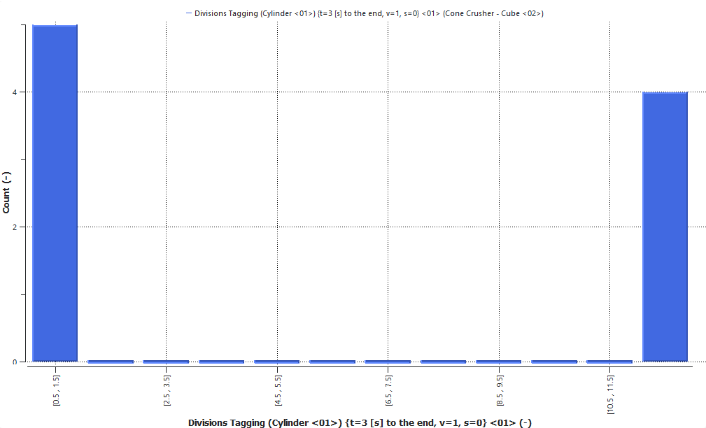
From the Histogram, it can be seen that most of the accumulated Fragments are coming from bins 1 and 12 of the hopper.
This information may not have been obvious before the Divisions Tagging analysis. Now, an appropriate solution can be devised if this particular result is undesirable.
It might also be useful to filter out the particles that actually broke; in Rocky, these broken particles are called fragments.
One way to isolate these fragments is by using the Laguerre-Vonoroi Size property, which has the following characteristics:
It is measured only for breakage fragments.
It is equal to the diameter of a sphere used to generate the fragments using the Laguerre-Voronoi tessellation.
This diameter,
 , can be defined as twice the minimum distance between a particle's
center of gravity,
, can be defined as twice the minimum distance between a particle's
center of gravity,  , and the particle's sides,
  , as shown in the following equation:
(8–1)
Using this property, the particles that did not break will have values equal to zero.
Therefore, to filter out only the fragments, we will select only the particles that have a Laguerre-Vonoroi Size value greater than zero.
Let's start by creating the Filter User Process.
Use the information in the table below.
Step Data Entity Editors Location Parameter or Action Settings A Particles Create a Filter User Process B User Processes ﹂Filter <01>
Property Property Laguerre-Voronoi Size ⯆ Type Range ⯆ Minimum Value 1e-10 [m] Maximum Value 0.2 [m]
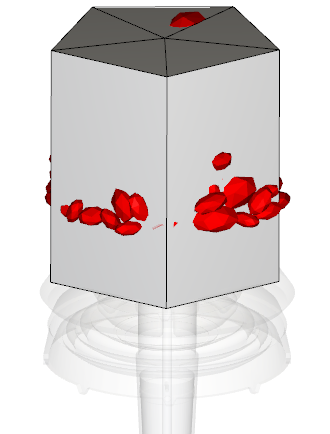
Then, to visualize in a 3D View window only the filtered fragments:
Select a 3D View window (or create a new one by pressing Ctrl + D).
Ensure the geometries are transparent (or hidden).
From the Data panel, hide Particles and all other Particles Calculations and User Processes (besides Filter <01>) using the eye icons.
From the Data Editors panel, on the Filter <01> entity, select the Properties tab, and then drag and drop Laguerre-Vonoroi Size onto the 3D View window. (Results shown below.)
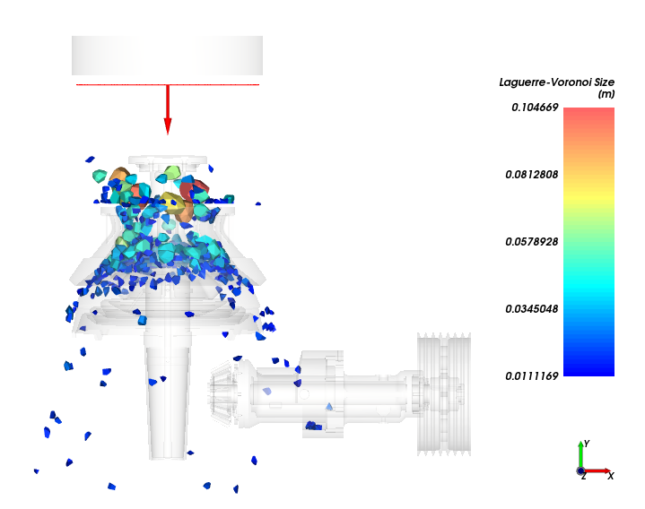
The view now shows only the particles that have broken (fragments).
Earlier in Part A, we turned on the collection of some Boundary Collision Statistics; specifically, those regarding Intensities.
We can now use the resulting data to estimate how much power is required by the equipment, which is commonly known as Power Draw.
The Average Power Draw of the geometries can be estimated by the following expression:
 | (8–2) |
where:
 is the output time.
  is the Average Power Draw at the
current output time.
is the Average Power Draw at the
current output time.  is the output time in which the operating conditions begin.
  is the output time in which the analysis ends.
  is the Output Frequency.
First, let's define .
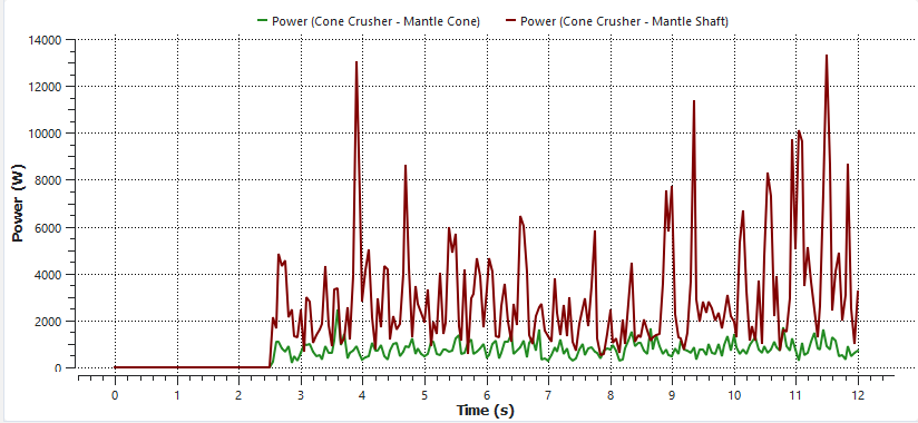
Use the information in the table below to plot the power curves for the cone and shaft geometries.
Step Data Entity Editors Location Parameter or Action Settings A Geometries ﹂Mantle Cone
Curves | Power Show Curve in New Plot B Geometries ﹂Mantle Shaft
Drag and Drop onto Time Plot <01> window
The plot shows the operation conditions start after 2.5 seconds (in which the breakage
starts), so = 2.5s.
Now, let's apply the Average Power Draw formula to the Power curve.
Use the information in the table below to continue with the analysis.
Step Item Location Parameter or Action Settings A Geometries ﹂Mantle Shaft
Curves Add new custom curve (button) B Add new (dialog box)
Name Average Power Output unit W Inputs | Power (Enabled) C Custom Curves (dialog box) Expression cumsum(A)*OUTPUT_FREQUENCY/(TIME_ELAPSED-2.5)
The new Average Power (Custom) curve appears on the Curves tab for the selected geometry, but is also made available for all other geometries automatically.
Now, let's sum the Average Power of the Mantle Cone and the Mantle Shaft geometries to estimate the Average Power Draw of the equipment:
Use the information in the table below to continue with the analysis.
Step Item Location Parameter or Action Settings A Geometries ﹂Mantle Cone
Curves | Average Power (Custom) Show curve in new plot B Geometries ﹂Mantle Shaft
Drag and drop onto open Time Plot <02> window C Time Plot <02> (window) Table (tab) Add Formula D Add Expression (dialog box) Curve Caption Average Power Draw Curve Expression B+C
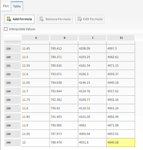
Each row of this table shows the average power measured from 2.5s to the time shown in Column A.
Thus, the Average Power Draw of the simulation is in the last row of this table and it is 4840.28 W (as shown).
Note: The values you end up with in your project may vary slightly from the ones shown in this Tutorial.
This completes Part B of this tutorial, in which Rocky was used to analyze the results from a cone crusher simulation.
During this tutorial, it was possible to:
Use Cube and Particles Time Selection User Processes to plot the PSD of fragments in a Histogram.
Use a Cylinder User Process and Divisions Tagging Particle Calculations to track specific particles and fragments through the equipment.
Use the Property User Process and the Laguerre-Voronoi Size Property to isolate the particle fragments from the whole particles.
Use the Intensities Boundary Collision Statistics data we collected to calculate the power draw.
What's Next?
If you completed this tutorial successfully, then you are ready to move on to next tutorial.