


(Part A) Learn how to set up and process a simulation using periodic motions, replicated geometries and periodic injection of material.
(Part B) Learn how to analyze the trajectories of the particles from the periodic injection, as well as the mass flow during surge periods and the mass load in each bucket.
The purpose of this tutorial is to learn how to use periodic motions with replicated geometries.
The scenario considered is a bucket conveyor experiencing surges of material from inconsistent loading.
We will post-process the results of this simulation in Part B.
You will learn how to:
Define a motion that can be repeated on a periodic basis
Replicate a geometry component multiple times along a defined path
Simulate a surge loading scenario by using periodic injection
And you will use these features:
Inlets
Periodic Motion
Geometry Replication
Periodic Injection
Important: This ADVANCED tutorial contains fewer details, screenshots, and procedures than other Rocky tutorials.
An ADVANCED tutorial is designed for users who are more familiar with the Rocky user interface (UI), and already have a good understanding of the common setup and post-processing tasks.
If you do not already have this level of familiarity, it is recommended that you complete at least Tutorials 01- 05 before beginning this one.
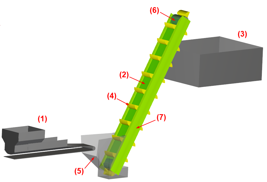
The geometries in this tutorial are composed of:
(1) Feed Conveyor
(2) Belt
(3) Box
(4) Bucket
(5) Hopper
(6) Rolls
(7) Structure
The first item will be created from a Rocky conveyor template.
The remaining components will be imported as .stl files, all of which can be found in the tutorial directory.
To get started with this tutorial, do the following:
Download the
dem_tut10_files.zipfile here .Unzip
dem_tut10_files.zipto your working directory.Open Rocky 2025 R2.
Create a new project.
Save the empty project to a location of your choosing.
Use the information in the table below to start setting up your Rocky project.
Step Data Entity Editors Location Parameter or Action Settings A Study Study Study Name Bucket Conveyor B Physics Physics | Momentum Rolling Resistance Model Type C: Linear Spring Rolling Limit ⯆ Numerical Softening Factor 0.1 [ - ] Tip: If you run into settings or procedures in these tables that you are not yet familiar with, please refer to the Rocky User Manual and/or other Tutorials (via the Introductory Tutorials and Advanced Tutorials) to find the detailed instructions you need.
For the Geometries step, we will import the following 6 geometry files in .stl format:

We will also add a default Feed Conveyor, and then create two separate Inlets (from two different Surfaces) from which to release the regular and surge material, respectively.
Use the information in the table that follows to import and create these components.
Step Data Entity Editors Location Parameter or Action Settings A Geometries Import Wall All 6 .stl files with "mm" for Import Unit B Geometries Create Feed Conveyor C Geometries ﹂Feed Conveyor <01>
Feed Conveyor | Geometry
Transition Length 1 [m] Loading Length 2 [m] Belt Width 0.5 [m] Belt Thickness 0.0125 [m] D Geometries ﹂Feed Conveyor <01>
Feed Conveyor | Orientation
Alignment Angle 90 [dega] Vertical Offset 0.6 [m] Horizontal Offset -0.07 [m] Out-of-plane Offset 0.95 [m] E Feed Conveyor | Skirtboard
Width 0.45 [m] Length 1.5 [m] Skirtboard Height 0.2 [m] Length Offset 0.5 [m] F Feed Conveyor | Feeder Box
Drop Box Length 1 [m] Drop Box Width 0.75 [m] Drop Box Height 0.25 [m] Wall Thickness 0.00625 [m] G Feed Conveyor | Head Pulley
Face Width 0.5 [m] Diameter 0.1 [m] H Geometries ﹂Feed Conveyor <01>
Feed Conveyor | Belt Motion
Belt Speed 0.75 [m/s] I Geometries Create Rectangular Surface J Geometries ﹂Rectangular Surface <01>
Rectangular Surface Name Regular Feed Center Coordinates -0.05, 1.6, 3.2 [m] Length 0.7 [m] Width 0.55 [m] Orientation Angles ⯆ Rotation 310, 0, 0 [dega] Tip: For more information about setting up Feed Conveyors, refer to Tutorial 06 – High Pressure Grinding Roll (HPGR).
From the Data panel, under Geometries, right-click Regular Feed and then click Duplicate.
Use the information in the table that follows to define the new Regular Feed <01> component.
Step Data Entity Editors Location Parameter or Action Settings K Geometries ﹂Regular Feed <01>
Rectangular Surface Name Surge Feed Center Coordinates -0.05, 1.6, 3.75 [m] Rotation 50, 0, 0 [dega]
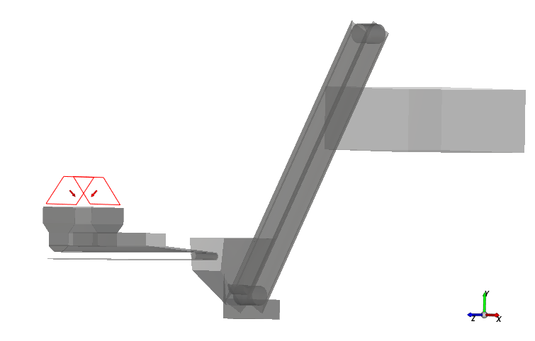
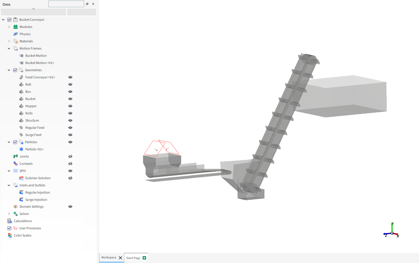
Now that all of the geometries are included in your project, you can visualize them in a 3D View window.
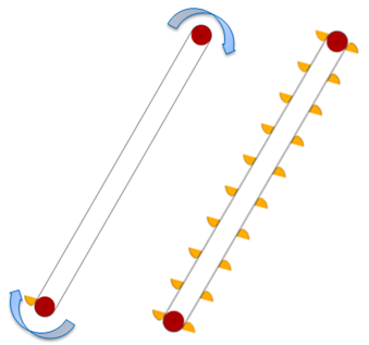
Turning the geometry for a single bucket into a full, 20-bucket conveyor involves the following steps:
(1) The complex motion of the single bucket moving up and around the conveyor is defined using a single motion frame.
(2) Periodic motions are turned on for this frame, which enables the entire motion set to be repeated at a prescribed interval.
(3) The motion frame is assigned to the bucket geometry.
(4) Rocky is then instructed to repeat the geometry (including its assigned motions) 20 times at regular intervals along the motion path.
For the Motion Frames step, we will accomplish the first two steps above by creating a single frame with four separate motions, as explained below.
The complex bucket motion can be defined on a single frame using four separate motions:
The translation motion of the right-side-up bucket moving up the front side of the conveyor.
The rotation motion of the bucket arching over the top of the conveyor to turn upside down.
The translation motion of the upside-down bucket moving down the back side of the conveyor.
The rotation motion of the upside-down bucket arching over the bottom of the conveyor to turn right-side up again.
The fourth motion brings the bucket back to the starting point, so to keep the bucket moving, the entire, four-part motion set must be repeated.
In Rocky, this motion repetition is done via Periodic Motions.
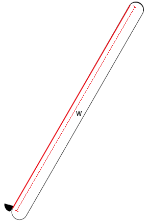
The four separate motions within the frame will be defined using the bucket velocity and belt length.
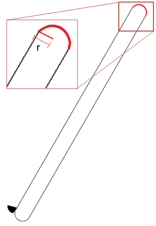
Important: Note that the full bucket motion includes two straight paths and two curved paths.
The bucket velocity: 1.15 m/s
The length of the straight path (w): 4.66174 m
The radius of the curved path (r): 0.15999 m
The bucket takes 4.05368 s to complete the straight path and 0.43706 s to complete the curved path
Using this information, we can then determine that one full revolution takes 8.98148 s.
Note: This value will be important both when setting up Periodic Motions and Geometry Replications later.
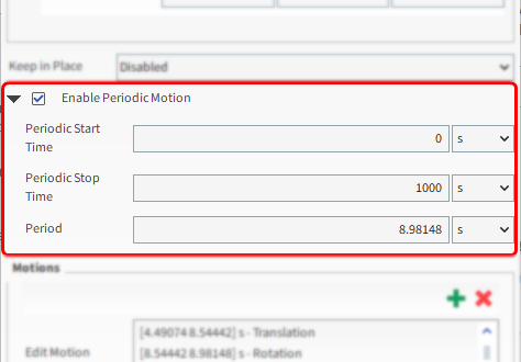
When Enable Periodic Motion is turned on for a frame, the full list of motions contained within that frame will be repeated as soon as the Periodic Motion Period completes.
The total time between the earliest motion's Start Time (in our case, 0 s) and the latest motion's Stop Time (in our case, 8.98148 s) is saved within Rocky as the periodic motion period.
As we want the motion to repeat as soon as the last motion finishes, we will set the Periodic Motion Period as equal to the motion total time.
The full list of motions contained within the frame will be repeated until it reaches the Periodic Stop Time.
Now that you understand more about periodic motions, you can create the single motion frame that will contain the four separate bucket motions.
Use the information in the table that follows to define this Motion Frame, and assign it to the bucket geometry.
Step Data Entity Editors Location Parameter or Action Settings A Motion Frames Create Motion Frame B Motion Frames ﹂Frame <01>
Frame Name Bucket Motion Relative Orientation | Angle -30 [dega] Enable Periodic Motion (Enabled) Period 8.98148 [s] Add Motion Stop Time 4.05368 [s] Velocity 0, 1.15, 0 [m/s] C Motion Frames ﹂Bucket Motion
Frame Add motion (2 of 4) Start Time 4.05368 [s] Stop Time 4.49074 [s] Type Rotation ⯆ Initial Angular Velocity -7.18794, 0, 0 [rad/s] Add motion (3 of 4) Start Time 4.49074 [s] Stop Time 8.54442 [s] Velocity 0, 1.15, 0 [m/s] Add motion (4 of 4) Start Time 8.54442 [s] Stop Time 8.98148 [s] Type Rotation ⯆ Initial Angular Velocity -7.18794, 0, 0 [rad/s] D Geometries ﹂Bucket
Wall Motion Frame Bucket Motion ⯆
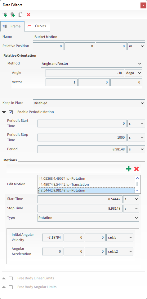
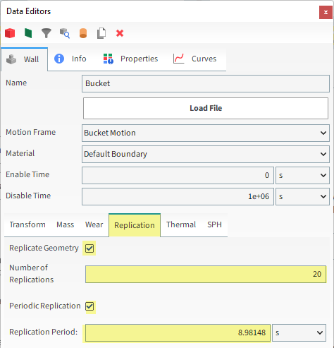
The completed Motion Frame setup should now look similar to the image below.
For this tutorial, since the geometry has a motion with displacement assigned, the movement can be previewed using the Motion Preview window.
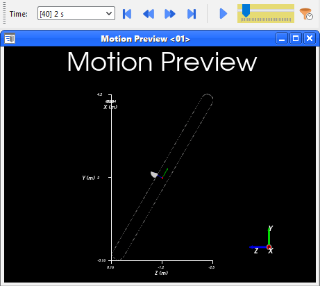
Tip: Use the eye icons on the Data panel to hide all but the Bucket and Belt components from the view.
Later in Part B of this tutorial we will analyze two buckets separately using moving cubes.
Note: A moving cube is a definition for a Cube User Process with a Motion Frame assigned to it.
Motions must be created before processing any simulation.
Follow the steps in the table below to create the second Motion Frame.
| Step | Data Entity | Editors Location | Parameter or Action | Settings |
|---|---|---|---|---|
| A | Motion Frames ﹂Bucket Motion | Duplicate Motion Frame | ||
| B | Motion Frames ﹂Bucket Motion <01> | Frame | Relative Position | 0, 4.04, -2.33 [m] |
| Relative Orientation | Angle | -210 [dega] | |||
For this tutorial, the Replicate Geometry option will be activated for the Bucket geometry, which will create copies of the geometry (and its assigned motions) at specified intervals along the motion's path.
From the Data panel, under Geometries, select Bucket.
From the Data Editors panel, select the Wall | Replication tab, and then enable the Replicate Geometry checkbox.
Define the Number of Replications value.
Enable the Periodic Replication checkbox.
To have the buckets appear in the correct location, enter the full periodic motion period (8.98148 s) for the Replication Period.
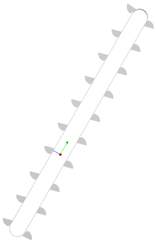
The results are shown below.
As seen in the Motion Preview (and/or 3D View) window, the single bucket has now been replicated into 20 buckets evenly spaced along the path of the bucket motion.
For the Materials step, default values will be used for all three default materials.
We will slightly modify the friction values for the Materials Interactions step.
And for the Particles step, we will create a new sphere-shaped particle group in a range of sizes with some added rolling resistance.
Use the information in the table below to continue setting up your project.
Step Data Entity Editors Location Parameter or Action Settings A Materials Interactions … | Default Particles⯆
Default Boundary⯆
Static Friction 0.5 [ - ] Dynamic Friction 0.5 [ - ] B Particles Create Particle C Particles ﹂Particle <01>
Particle | Size Add size row (x1) (1) Size | Cumulative % 0.15 [m] @ 100 [%] (2) ... 0.05 [m] @ 10 [%] Particle | Movement Rolling Resistance 0.4 [ - ]
For the Inlets and Outlets step, we will create two particle inlets: one to provide a consistent feed for the conveyor and another to provide additional surges of material through the inlet.
Use the information in the table below to create the first inlet representing the regular feed.
Step Data Entity Editors Location Parameter or Action Settings A Inlets and Outlets Create Particle Inlet B Inlets and Outlets ﹂Particle Inlet <01>
Particle Inlet Name Regular Injection Entry Point Regular Feed ⯆ Particle Inlet | Particles Add row (x1) (1) Particle | Mass Flow Rate Particle <01> ⯆ @ 70 [t/h]
For the second inlet, we want the material surge to be represented by 5-second bursts of material that appear every 5 seconds, starting 5 seconds into the simulation (as shown).
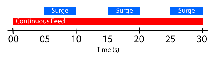
To replicate the material surge, we will set this second Particle Inlet to have a Periodic injection, which will enable particles to be released from the Entry Point in bursts.
These bursts are defined via the following parameters:
Period: Defines the length of time for each injection cycle.
Injection Duration: Defines the amount of time during each Period when particles will be actively released.
Rocky calculates the particle mass released in each periodic burst by equally dividing the total particle mass by the total number of bursts during the simulation.
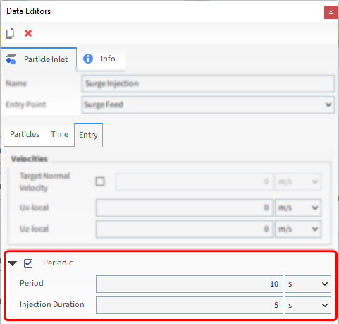
Use the information in the table below to create a second Particle Inlet for the material surge, and to complete your simulation setup.
Step Data Entity Editors Location Parameter or Action Settings A Inlets and Outlets Create Particle Inlet B Inputs ﹂Particle Inlet <01>
Particle Inlet Name Surge Injection Entry Point Surge Feed ⯆ Particle Inlet | Particles Add row (x1) (1) Particle | Mass Flow Rate Particle <01> ⯆ @ 40 [t/h] … | Time Start 5 [s] … | Entry Periodic (Enabled) Periodic | Period 10 [s] Periodic | Injection Duration 5 [s] C Solver Solver | Time Simulation Duration 30 [s] Solver | General Simulation Target CPU ⯆
With a 3D View window opened, your Data panel and Workspace should look similar to the below image.
From the Solver entity, click Start.
The Simulation Summary screen appears, then processing begins.
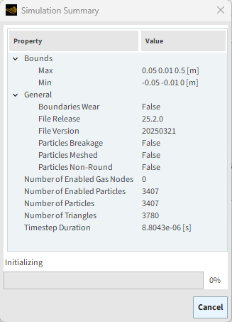
Tip: You can use the Auto Refresh checkbox to view in a 3D View window the results during processing.
This completes Part A of this tutorial, in which Rocky was used to set up and process a simulation of a Bucket Conveyor.
During this tutorial, it was possible to:
Define a motion that repeats periodically
Replicate a single geometry into multiple copies with identical motion paths
Set up a material surge scenario using a periodic injection inlet
What's Next?
Now that you have set up and processed this simulation, you are ready to move on to Part B and post-process this project.
The purpose of this tutorial is to analyze the results from the Bucket Conveyor simulation we processed in Part A.
You will learn how to:
Visualize the two separate injections
Evaluate the mass flow during the surge periods
Evaluate the mass load for each bucket that has reached a steady state
Analyze the trajectory of the particles being dumped into the bin
And you will use these features:
3D View
User Processes (Cube, Particle Trajectory)
Time Plot and Custom Formulas
Important: This ADVANCED tutorial contains fewer details, screenshots, and procedures than other Rocky tutorials.
An ADVANCED tutorial is designed for users who are more familiar with the Rocky user interface (UI), and already have a good understanding of the common setup and post-processing tasks.
If you do not already have this level of familiarity, it is recommended that you complete at least Tutorials 01- 05 before beginning this one.
If you completed Part A of this tutorial, ensure that Rocky project is open. (Part B will continue from where Part A left off.)
If you did not complete Part A, do all of the following:
Download the
dem_tut10_files.zipfile here .Unzip
dem_tut10_files.zipto your working directory.Open Rocky 2025 R2.
Important: To make use of the Rocky project file provided, you must have Rocky 2025 R2 or later. If you have an earlier version of Rocky, please upgrade Rocky to the latest version, or complete Part A from scratch.
From the Rocky program, click the Open Project button, find the dem_tut10_files folder, then from the tutorial_10_A_pre-processing folder, open the tutorial_10_A_pre-processing.rocky file.
Process the simulation. (From the Data panel, select Solver and then from the Data Editors panel, click the Start button.)
Now that our project has finished processing, we can begin analyzing the results.
Let's start by viewing the contributions from each separate inlet.
From the Data panel, select Particles.
From the Data Editors panel, on the Properties tab, right-click Particle Boundary, point to 3D View, and then click Show in new 3D View.
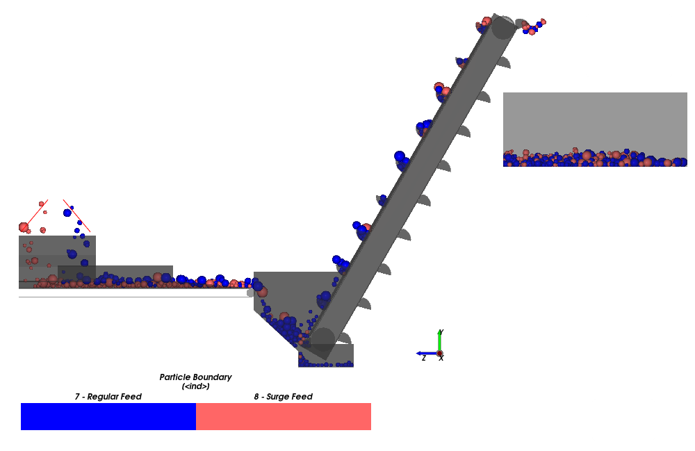
Each inlet's contribution is represented by a separate color.
Note: Particle boundaries are numbered from zero in the order in which they were added to the Geometries entity.
Tip: Use the slider on the Time toolbar to investigate the surges at different times.
Another way to evaluate the effect of the surges is to plot the particles count.
From the Data panel, select Particles again.
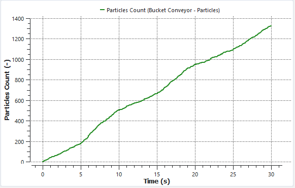
From the Data Editors panel, on the Curves tab, drag and drop Particles Count onto the Workspace.
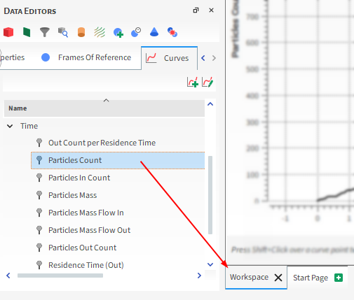
The resulting plot shows a steeper curve whenever the mass flow is increased from a surge.
We can also filter the particles by the Particle Boundary property and plot the Particles Count for each Inlet separately.
First we will isolate the particles that result from the Regular Feed.
Use the information in the table below to begin this analysis.
Step Data Entity Editors Location Parameter or Action Settings A Particles Create a Filter User Process B User Processes ﹂Filter <01>
Property Name Regular Feed Particles Property Particle Boundary ⯆ Type Value Cut value 7 [<ind>] Next, we will isolate the particles that result from the Surge Feed.
From the Data panel, under User Processes, right-click Regular Feed Particles, and then click Duplicate.
Use the information in the table below to define the newly created Regular Feed Particles <01> item.
Step Data Entity Editors Location Parameter or Action Settings A User Processes ﹂Regular Feed Particles <01>
Property Name Surge Feed Particles Cut value 8 [<ind>] Now, from the Data panel, under User Processes, multi-select both Regular Feed Particles and Surge Feed Particles.
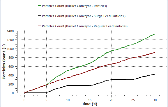
Drag-and-drop both processes onto the previous plot.
The resulting plot shows two more curves:
The Surge Feed is represented by a "stairstep" curve that shows the different periods of injection over time.
The Regular Feed is represented by a curve that grows at constant rate.
Next, let's evaluate the draw efficiency.
This can be done by using two moving cubes (each one for a bucket) and a Time Plot to analyze the carried Particle Mass for each bucket.
We will use the motion frames we created in Part A to describe the cubes motion.
Use the information in the table below to create the moving cubes.
Step Data Entity Editors Location Parameter or Action Settings A Particles Create a Cube User Process B User Processes ﹂Cube <01>
Cube Motion Frame Bucket Motion ⯆ Center -0.06, 0.27, 0.2 [m] Magnitude 0.5, 0.5, 0.3 [m] Orientation | Method Angles ⯆ Orientation | Rotation -30, 0, 0 [m] C User Processes ﹂Cube <01>
Duplicate Cube User Process D User Processes ﹂Cube <02>
Cube Motion Frame Bucket Motion <01> ⯆ Center -0.06, 3.8, -2.55 [m]
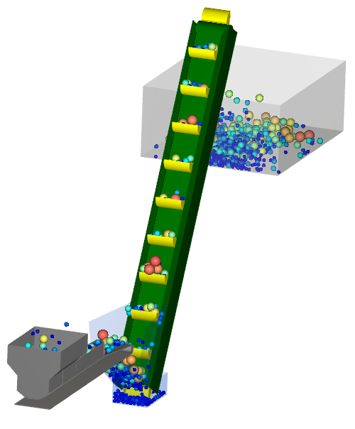
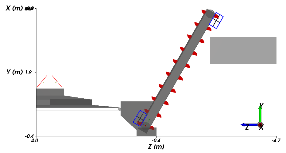
This results in two cubes encompassing two buckets (as shown).
Due to the assigned motion frames, the cubes will accompany the buckets for the whole simulation (check this on Motion Preview and by multi-selecting both cubes with the Bucket wall visible).
Now that we have the Cube selections, we can use it to create a Time Plot showing the Sum of Particle Mass for the two buckets.
Use the information in the table below to create the Time Plot.
Step Item Location Parameter or Action Settings A Window (menu) Create a New Time Plot B Cube <01> Properties | Particle Mass Drag and drop onto the Time Plot window C Select the Statistics to Plot (dialog box) Sum (Enabled) (All others) (Cleared) D Cube <02> Properties | Particle Mass Drag and drop onto the Time Plot window E Select the Statistic to Plot (dialog box) Sum (Enabled) (All others) (Cleared)
The resulting plot represents the Particle Mass in each Cube region.

Note: Each bucket we are analyzing pass through the Hopper 3 times.
Note that when crossing the Hopper (at 13.3 s for example), the cubes encompass particles that are not necessarily being carried by the buckets, and it causes peaks on the plot.
The relevant values are the ones that keep constant for more than a second in the plot, when all the particles inside the cube are being carried by the bucket (15 s). (Compare the images shown.)
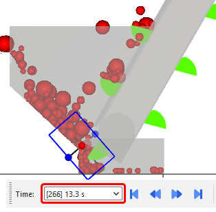
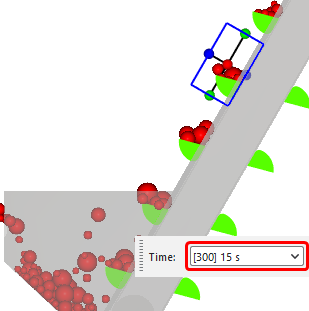
The particle mass carried by the buckets varies between 2.6 kg (at the beginning, with few particles on the Hopper) and 16 kg.
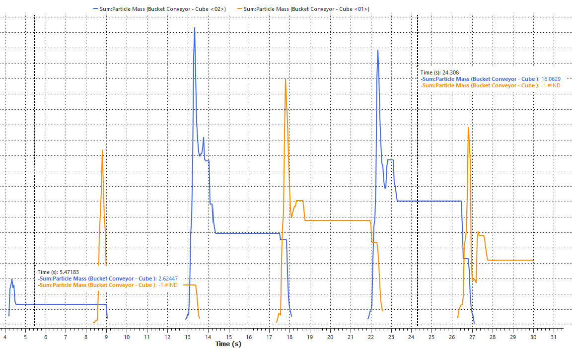
Note: Your values may differ slightly from the ones presented in this tutorial.
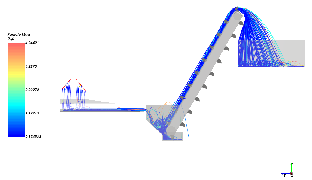
Another analysis we can do with this project involves using the Particles Trajectory User Process, which displays the path particles take by translating their movements into 3D curves.
Tip: To learn more about Particle Trajectories, refer to Tutorial 04 – SAG Mill Tutorial - SAG Mill.
To visualize the trajectory of the particles, do the following:
From the Time toolbar, ensure that you have selected the [120] 6 s timestep. This will be your Starting Timestep.
Use the information in the table below to create the Particles Trajectory.
Step Data Entity Editors Location Parameter or Action Settings A Particles Create a Particles Trajectory User Process B User Processes ﹂Particles Trajectory <01>
Particle Trajectory Number of Intervals 300 [ - ] Particle Stride 1 [ - ] Update Particles Selection Your Starting Timestep value should be updated accordingly.
To view the trajectories, use the information in the table below.
Step Item Location Parameter or Action Settings A Window (menu) Create a New 3D View B User Processes | Particles Trajectory <01>
Coloring Visible (Enabled) Edges (Enabled) Edges | Property Particle Mass ⯆
Tip: Hide Particles from the view by using its Data panel eye icon.
This completes Part B of this tutorial, in which Rocky was used to analyze the results from a Bucket Conveyor simulation.
During this tutorial, it was possible to:
Visualize and plot the effects of the two separate injections
Evaluate the mass load for a single bucket using Cubes and Time Plots
Visualize the trajectory of the particles
What's Next?
If you completed this tutorial successfully, then you are ready to move on to the next tutorial.