

(Part A) Set up and process a simulation with coupled SPH and DEM.
(Part B) Learn how to analyze the power supply of the system and the influence of the slurry filling.
The main purpose of this tutorial is to:
Set up and process an SPH-DEM coupled simulation.
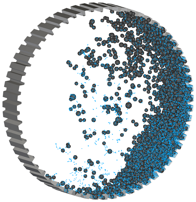
The scenario considered in this simulation is a Slurry Mill.
In wet milling, the presence of slurry (fluid mixture) can affect the supplied power.
You will learn how to:
Set up a SPH-DEM case
Use the same Volumetric inlet to inject both DEM and SPH
Enable the collection of SPH Boundary Interaction Statistics
And you will use these features:
SPH
Modules
Inlets and Outlets - Volumetric Inlet
Cartesian Periodic Domains
Important: This ADVANCED tutorial contains fewer details, screenshots, and procedures than other Rocky tutorials.
An ADVANCED tutorial is designed for users who are more familiar with the Rocky user interface (UI), and already have a good understanding of the common setup and post-processing tasks.
If you do not already have this level of familiarity, it is recommended that you complete at least Tutorials 01 - 05 before beginning this one (especially Tutorial - SAG Mill, which has the same context of this one but without fluid injection).

The geometry in this tutorial is composed of:
Mill slice
In the tutorial directory, the .stl file can be found.
To get started with this tutorial, do the following:
Download the
dem_tut25_files.zipfile here .Unzip
dem_tut25_files.zipto your working directory.Open Rocky 2025 R2.
Create a new project.
Save the empty project to a location of your choice.
Tip: If you run into settings or procedures in these tables that you are not yet familiar with, please refer to the Rocky User Manual and/or other Tutorials to find the detailed instructions you need.
Let's begin our setup by defining Physics and Modules parameters.
Use the information in the table that follows to start setting up your Rocky project.
Step Data Entity Editors Location Parameter or Action Settings A Study Study Study Name Slurry Mill B Physics Physics | Momentum Rolling Resistance Model Type C: Linear Spring Rolling ⯆ Numerical Softening Factor 0.1 [ - ] C Modules Modules Boundary Collision Statistics (Enabled) SPH Boundary Interaction Statistics (Enabled) D Modules ﹂Boundary Collision Statistics
Boundary Collision Statistics Intensities (Enabled) E Modules ﹂SPH Boundary Interaction
SPH Boundary Interaction Statistics Power (Enabled)
Note: By enabling the checkboxes from Steps D and E, the modules will collect interaction data (with the particles and fluid) for the boundaries that we will use later to calculate the power draw of the Mill.
For this tutorial, start up and steady state Rotation motions within the same Frame will be created for the Mill.
Follow the steps in the table below to import the mill slice geometry and create the Motion Frame that will be attached to it later.
Step Data Entity Editors Location Parameter or Action Settings A Geometries Import Wall Mill.stl with "mm" for Import Unit B Motion Frames Create Motion Frame C Motion Frames ﹂Frame <01>
Frame Name Rotation Motion Add motion Stop Time 3 [s] Type Rotation ⯆ Angular Acceleration 0, 0, 200 [rev/min] Add motion Start Time 3 [s] Type Rotation ⯆ Initial Angular Velocity 0, 0, 10 [rev/min]
Next, we will assign the created Motion Frame to the Mill.
We will also set the Triangle Size in order to be refined but not excessively fine to balance resolution with computational time.
Use the information in the table below to continue your setup.
Step Data Entity Editors Location Parameter or Action Settings A Geometries ﹂Mill
Wall Motion Frame Rotation Motion ⯆ … | Transform Triangle Size 0.5 [m]
To visualize the Mill movement, preview it in a Motion Preview window.
For the Materials step, default values for the boundaries (Default Boundary) will be used, we will create two new materials for Rock and Steel particles that will be inputed later and we will use the Default Fluid to represent the Slurry.
Note: In practice, the slurry properties can vary depending on which components are added to the water. In this tutorial, for simplicity, we will use default (water) properties.
Use the information in the following tables to set up the Materials and Materials Interactions steps.
Step Data Entity Editors Location Parameter or Action Settings A Materials Create Solid Material B Materials ﹂Material <04>
Material Name Rock Material Density 2800 [kg/m3] C Materials ﹂Material <05>
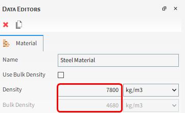
Material Name Steel Material Density 7800 [kg/m3] D Materials ﹂Default Fluid
Fluid Material Name Slurry Material E Materials Interactions Rock Material - Rock Material Static Friction 0.8 [ - ] Dynamic Friction 0.8 [ - ] Restitution Coefficient 0.5 [ - ] Rock Material - Steel Material Static Friction 0.5 [ - ] Dynamic Friction 0.5 [ - ] Restitution Coefficient 0.5 [ - ]
We will create two particles sets to represent Rock Particles and Steel Particles.
Use the information in the table below to create both particle sets.
Step Data Entity Editors Location Parameter or Action Settings A Particles Create Particle (x2) B Particles ﹂Particle <01>
Particle Name Rock Particles Material Rock Material ⯆ Particle | Size Add row (x2) Size | Cumulative % 0.3 [m] @ 100 [%] Size | Cumulative % 0.25 [m] @ 70 [%] Size | Cumulative¨% 0.2 [m] @ 20 [%] … | Movement Rolling Resistance 0.35 [ - ] C Particles ﹂Particle <02>
Particle Name Steel Particles Material Steel Material ⯆ Particle | Size Size | Cumulative % 0.35 [m] @ 100 [%] … | Movement Rolling Resistance 0.35 [ - ]
For the SPH step, we will use default values for every parameter but the Element Size.
From the Data panel, select SPH, and from Data Editors panel, ensure the Fluid Material is defined as Slurry Material.
From the Kernel field, define the Element Size.
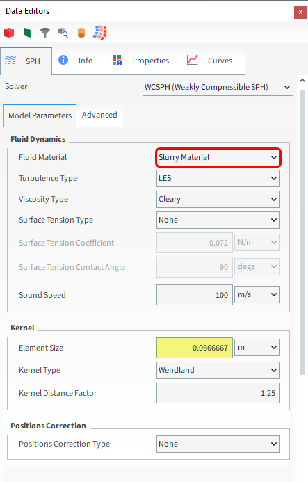
The Element Size is roughly 1/3 of the smallest Particle to ensure proper interaction between the SPH and DEM physics.
Refer to SPH Technical Manual for more information.
For this tutorial, we will create a single Volumetric Inlet to inject the Particle groups and SPH elements into the simulation.
Follow the steps in the table below in order to create and define the inlet.
Step Data Entity Editors Location Parameter or Action Settings A Inlets and Outlets Create Volumetric Inlet B Inlets and Outlets ﹂Volumetric Inlet <01>
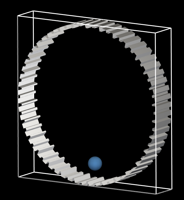
Volumetric Inlet | Particles Add row (x2) Particle | Mass Rock Particles ⯆ @32000 [kg] Particle | Mass Steel Particles ⯆ @ 8000 [kg] Volumetric Inlet | SPH Mass 8300 [kg] … | Region Seed Coordinates 0, -4, 0 [m] Geometries | Mill (Enabled) Use Geometries to Compute (Enabled)
In a 3D View it is possible to visualize the Region to be filled (white box) and the Seed (blue sphere) when the Inlet is selected.
For the Domain Settings step, we will define a Cartesian Periodic Domain to recycle particles and fluid that leave one side of the mill slice back into the simulation on the opposite side.
The same procedure for the Domain step is followed in the Tutorial 04. Refer to the tutorial and/or to the Rocky User Manual for more details about Periodic Domains.
For the Solver step, we will prefer to use a GPU in order to reduce the simulation time.
Follow the steps in the table below to set your Domain and Solver.
Step Data Entity Editors Location Parameter or Action Settings A Domain Settings Domain Settings Periodic Domain | Periodic Domain Type Cartesian ⯆ Periodic Domain | Periodic Direction | X (Cleared) Periodic Domain | Periodic Direction Z (Enabled) B Solver Solver | Time Simulation Duration 25 [s] Output Settings | Time Interval 0.1 [s] Solver | General Simulation Target GPU ⯆
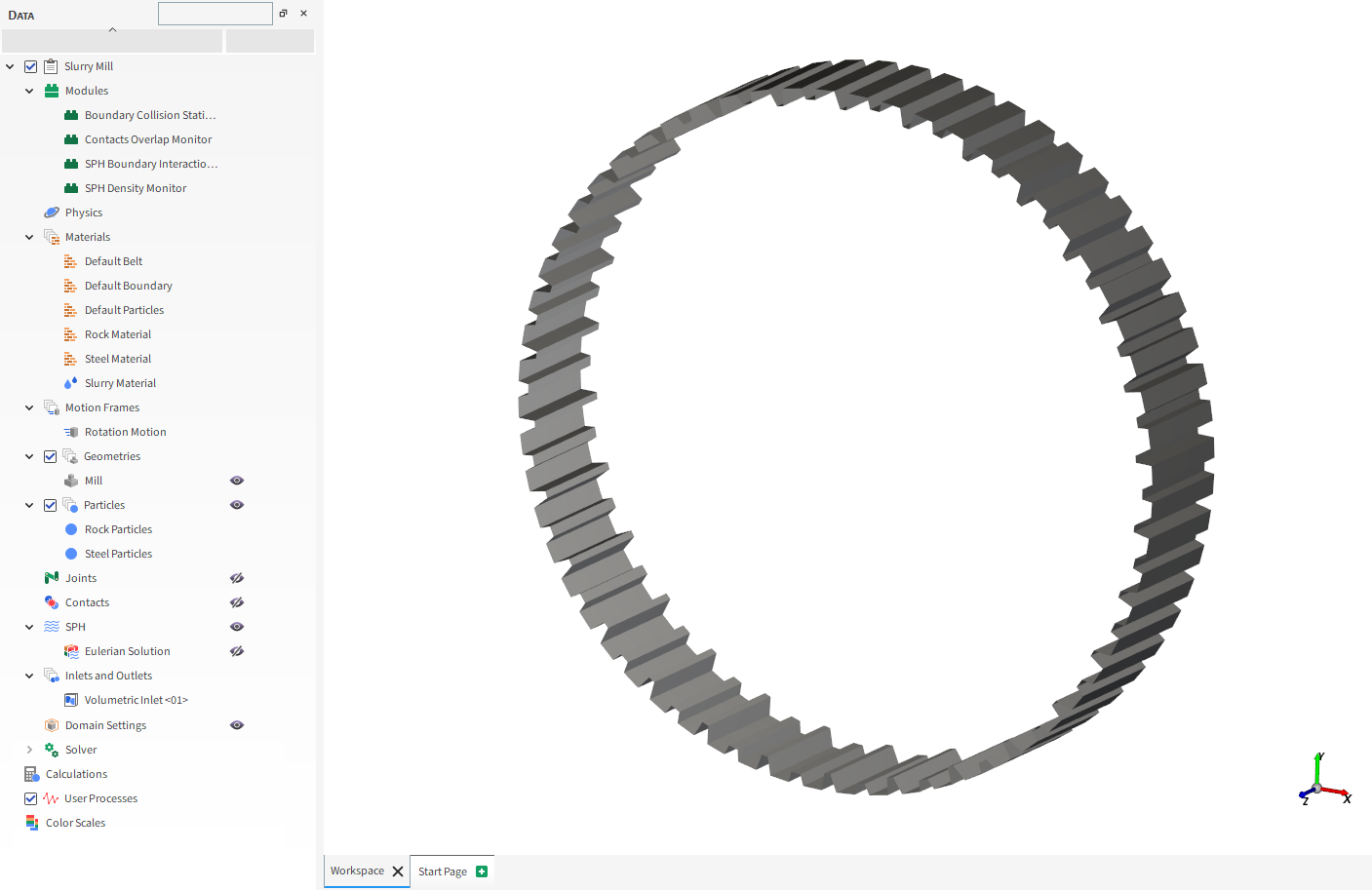
With a 3D View opened, your Data panel and Workspace should look similar to the image below.
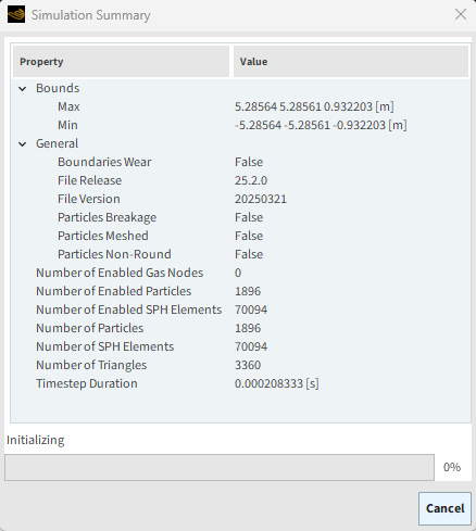
From the Solver entity, click Start.
The Simulation Summary appears (as shown), then processing begins.
This completes Part A of this tutorial, in which Rocky was used to set up and process a Slurry Mill simulation.
During this tutorial, it was possible to:
Enable Modules.
Define an Inlet for both particles and fluid.
Define a Periodic Domain.
What's Next? If you completed this tutorial successfully, then you are ready to move on to Part B and post-process this project.
The purpose of this tutorial is to analyze an SPH-DEM simulation of a Slurry Mill after you have processed it. We will continue from where we left off in Part A.
You will learn how to:
Evaluate mill Slurry Filling
Evaluate mill supplied power
Analyze pooling effects
And you will use these features:
Custom Properties
Expressions/Variables
Time Plot
Important: This ADVANCED tutorial contains fewer details, screenshots, and procedures than other Rocky tutorials.
An ADVANCED tutorial is designed for users who are more familiar with the Rocky user interface (UI), and already have a good understanding of the common setup and post-processing tasks.
If you do not already have this level of familiarity, it is recommended that you complete at least Tutorials 01 - 05 before beginning this one.
If you completed Part A of this tutorial, ensure that Rocky project is open. (Part B will continue from where Part A left off.)
If you did not complete Part A, do all of the following:
Download the
dem_tut25_files.zipfile here .Unzip
dem_tut25_files.zipto your working directory.Open Rocky 2025 R2.
Important: To make use of the Rocky project file provided, you must have Rocky 2025 R2 or later. If you have an earlier version of Rocky, please upgrade to the latest version, or complete Part A from scratch.
From the Rocky program, click the Open Project button, find the dem_tut25_files folder, and then from the tutorial_25_A_pre-processing folder, open the tutorial_25_pre-processing.rocky file.
Process the simulation. (From the Simulation toolbar, click the Start button.)
Our main interest in this tutorial is to evaluate the Supplied Power and analyze how it varies according to the Slurry Filling.
The Slurry Filling ( ) is the ratio between the volume of slurry
  loaded to the volume of particle interstices available within the bed at
rest, and it can be calculated using the following expression:
loaded to the volume of particle interstices available within the bed at
rest, and it can be calculated using the following expression:
 | (25–1) |
Where:
 is the static porosity of the bed of particles (≈ 0.360 - 0.42
on average)
is the static porosity of the bed of particles (≈ 0.360 - 0.42
on average)  is the mill volume fraction occupied by all particles (including the
interstices)
is the mill volume fraction occupied by all particles (including the
interstices)
Note:  represents the volume of particle interstices.
For this tutorial, we will assume = 0.4, as in reference paper [1].
The Slurry Filling can be analyzed so that:
- = 0: No slurry
0 <
< 1: Interstices partially filled - = 1: Interstices filled
- > 1: Slurry amount enough to fill the Interstices and left over
The parameters we need to calculate the Slurry Filling ( and ) can be obtained in Rocky (discussed below).
- : is the sum of the volumes of SPH
elements.
Note: The volume for a single SPH element is equal to Element Size cubed.
- : is the sum of the volumes of the
Particles (Particle Volume property) divided by the
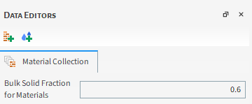
ratio between material Bulk Density and Density (to consider the interstices), that is 0.6 in Rocky by default (typical for spherical particles).
Let's calculate the Slurry Filling for our project.
Note: In the Part A of this tutorial, the Element Size and
SPH Mass (thus, the ) were intentionally chosen so that reaches approximately the unity ( ≈ 1).
Follow the steps in the table below to obtain the necessary parameters and calculate
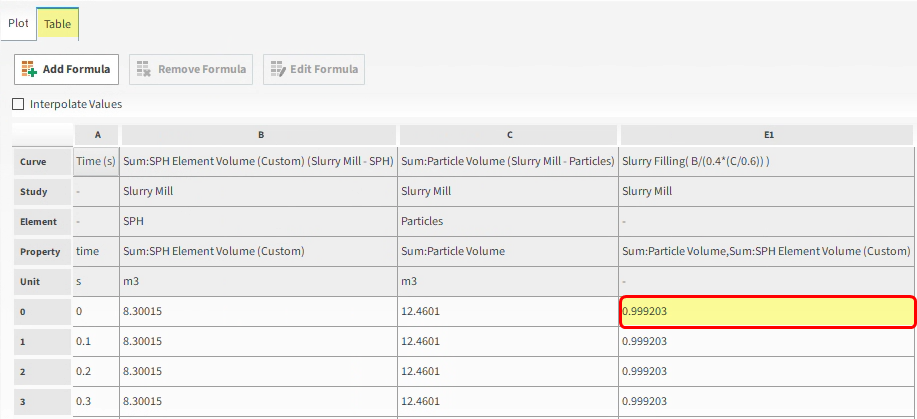
. Step Item Location Parameter or Action Settings A SPH Properties Add new custom property B Add new (dialog box) Name SPH Element Volume Output unit m3 C Custom Property (dialog box) Expression (2/30)**3 D SPH Properties | SPH Element Volume (Custom) Show in new Time Plot by Sum E Particles Properties | Particle Volume Show in selected Time Plot by Sum F Time Plot <01> Table Add Formula G Add Expression (dialog box) Curve Caption Slurry Filling Curve Expression B/(0.4*(C/0.6))
Note: For Step G, ensure B refers to SPH Element Volume (Custom) and C to Particle Volume.
You can visualize the resulting Slurry Filling in the Table tab from Time Plot <01>.
Note: The Slurry Filling depends on the static porosity of the
bed (), that must be evaluated with the bed of particles at rest.
Also note that for constant, the only parameter that would change the Slurry Filling value
in a simulation without fluid/particle inlets or outlets is the volume of slurry, due to
fluid compressibility, and these variations are not significant.
This way, Slurry Filling should be roughly constant for this simulation.
Tip: This analysis can be convenient when your simulation has slurry inlets or outlets.
Next we will evaluate and analyze the Supplied Power.
Note: The Supplied Power corresponds to the necessary energy for the Mill to maintain the prescribed rotational velocity. It accounts for the additional work to lift particles and fluid.
Tip: The Supplied Power has contributions from the fluid (SPH : Power) and Particles (Power), that have to be summed to represent it.
Follow the steps in the tables below to plot both the separated contributions and the Supplied Power.
Step Item Location Parameter or Action Settings A Geometries ﹂Mill
Curves Add new custom curve B Add new (dialog box) Name Supplied Power Output Unit W Inputs | Power (Enabled) Inputs | SPH : Power (Enabled) C Custom Curves (dialog box) Expression A+B D Geometries ﹂Mill
Curves | Power Show curve in new plot Curves | SPH : Power Show curve in selected plot Curves | Supplied Power (Custom) Show curve in selected plot On the Plot tab, make the Axes Layout By Quantity so you can easily visualize the difference between the Slurry and Particles influence in Supplied Power (results shown below).
The resulting plot is shown below. The black line represents the Supplied Power.
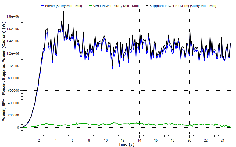
Note: The green line represents the portion of power consumed by the slurry.
Tip: If this curve becomes negative, it means that the slurry is contributing to the mill
rotation. In this tutorial, we will see when it happens and how to analyze it. It will
occur for some conditions with > 1.
In order to have a reference value for comparison purposes, lets calculate the average value for the Supplied Power with the mill at steady state.
Note: Later in this tutorial, results for different values of will be presented, and the procedures to get them are the same of the
ones presented in the following table.
Follow the steps in the table below to create a variable for the Supplied Power.
Step Item Location Parameter or Action Settings A Menu Tools Enable Expression/Variables B Geometries ﹂Mill
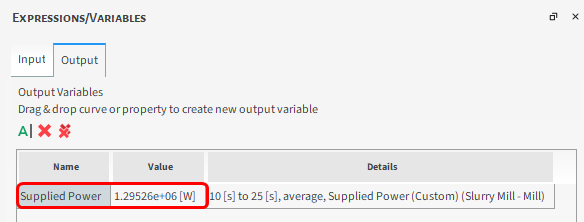
Curves | Supplied Power (Custom) Drag and drop to Expressions/Variables | Output From the Expressions/Variables panel, select Supplied_Power_Custom and click Edit.
Define the Name, Operation on Curve and Domain Range.
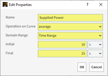
Click OK and see the resulting value on the Output tab.
An interesting phenomenon that starts to happen with a certain amount of Slurry in the Mill is pooling.
In this context, pooling is the formation of a slurry pool separated from the particles that contributes for the mill rotation by changing the center of gravity of the system.
Note: Therefore, it should be noted a Supplied Power reduction with the presence of pooling.
In the next section, we will visualize the slurry behavior for different values of
and check for which value the pooling starts for our setup.
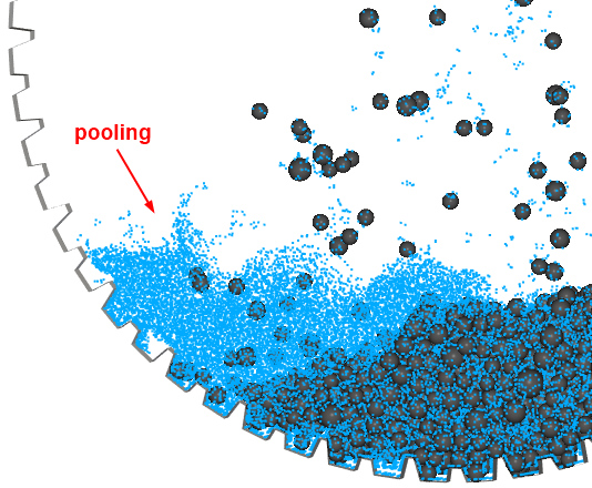
Example of pooling (
= 3)
Take a moment to analyze the slurry behavior for different Slurry Filling values (this and next section).
Note: These (07) 3D View results were obtained from the same setup of this tutorial for the last output, varying only the SPH Mass (slurry mass), indicated below each view.
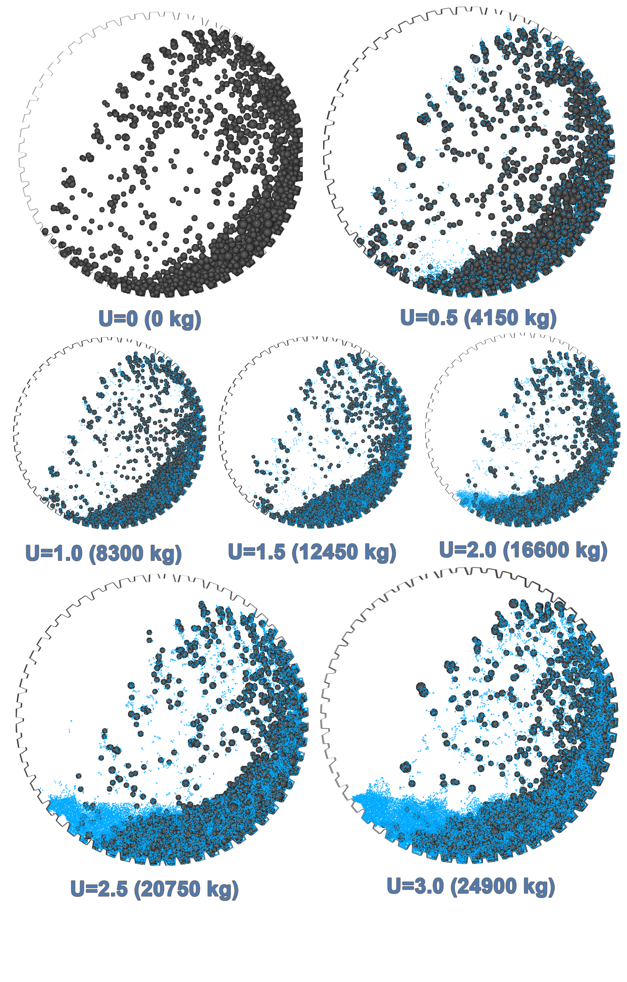
By following the procedures from POWER ANALYSIS for these 07 cases, it is possible to plot the Supplied Power as function of the Slurry Filling.
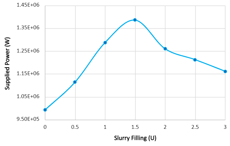
It is possible to see that the Supplied Power starts to reduce for > 1.5 as pooling takes place.
This completes Part B of this tutorial.
Rocky was used to analyze a Slurry Mill.
During this tutorial, it was possible to:
Set up a DEM-SPH simulation
Plot Curves and Properties
Visualize a comparison for different setups within the same mill