


(Part A) Project Setup and Processing
(Part B) Post-Processing
Note: This is an advanced tutorial.
The main purpose of this tutorial is to introduce SPH entity parameters and to process a fluid-only simulation in Rocky.
The scenario considered is a dam break.
You will learn how to:
Configure fluid material
Collect fluid collision data
Create a fluid inlet
And you will use these features:
SPH
SPH Boundary Interaction Statistics
Eulerian Solution
Inlets and Outlets
Important: This ADVANCED tutorial contains fewer details, screenshots, and procedures than other Rocky tutorials.
An ADVANCED tutorial is designed for users who are more familiar with the Rocky user interface (UI), and already have a good understanding of the common setup and post-processing tasks.
If you do not already have this level of familiarity, it is recommended that you complete at least Tutorials 01- 05 before beginning this one.
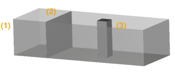
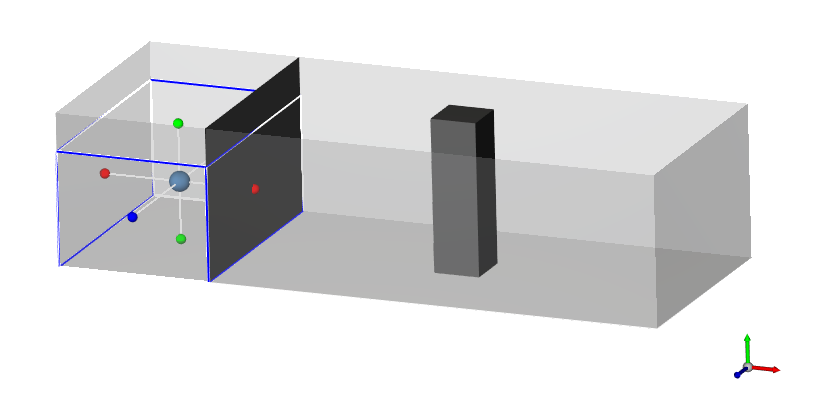
The wall geometries in this tutorial are composed of:
(1) container
(2) gate
(3) column
In the tutorial directory each .stl file can be found.
To get started with this tutorial, do the following:
Download the
dem_tut24_files.zipfile here .Unzip
dem_tut24_files.zipto your working directory.Open Rocky 2025 R2.
Create a new project.
Save the empty project to a location of your choosing.
Tip: If you run into settings or procedures in these tables that you are not yet familiar with, please refer to the Rocky User Manual and/or other Tutorials to find the detailed instructions you need.
Use the information in the table that follows to start setting up your Rocky project.
Step Data Entity Editors Location Parameter or Action Settings A Study 01 Study Study Name Dam Break B Modules Modules SPH Boundary Interaction Statistics (Enabled) C Modules ﹂SPH Boundary Interaction Statistics
SPH Boundary Interaction Boundary Properties | Nodal Forces (Enabled) Boundary Curves | Force (Enabled) D Geometries Import Wall column.stl, container.stl and gate.stl with "m" for Import Unit Note: By enabling the checkboxes from Step C, the module will collect force interaction data for the boundaries.
The Boundary Properties field enables values for each boundary triangle for each timestep, that you can make operations with.
The Boundary Curves field enables average values that correspond to the referred boundary for each timestep.
Make the three imported walls transparent to make the visualization better.
For this tutorial, one Translation movement will be created for the gate in order to release the water that will be filling the space limited by the container and gate.
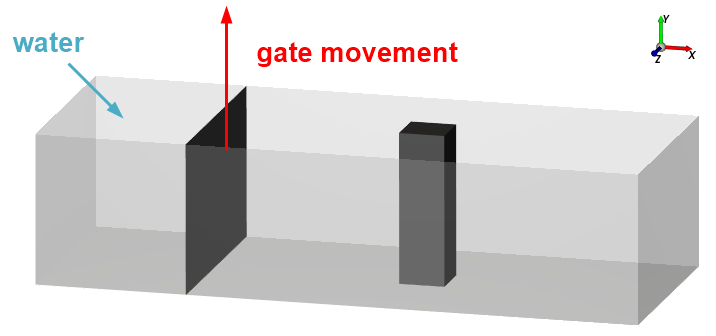
To create and assign the Motion Frame for the gate, follow the table below.
| Step | Data Entity | Editors Location | Parameter or Action | Settings |
|---|---|---|---|---|
| A | Motion Frames | Create Motion Frame | ||
| B | Motion Frames ﹂Frame <01> | Frame | Name | Gate Opening |
| Add Motion | ||||
| Motions | Start Time | 0.5 [s] | |||
| … | Stop Time | 0.9 [s] | |||
| … | Velocity | 0, 1, 0 [m/s] | |||
| C | Geometries ﹂gate | Wall | Motion Frame | Gate Opening ⯆ |
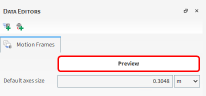
To visualize the gate movement, preview it in a Motion Preview window (from Motion Frames, click the Preview button).
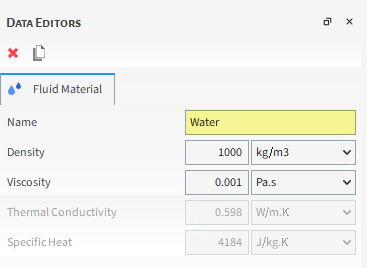
For the Materials step, default values for the boundaries (Default Boundary) will be used and we will set the Fluid Material to represent Water.
From the Data panel, under Materials, select Default Fluid and define the Name in the Data Editors panel.
The SPH step allows you to define the SPH Solver, Kernel, Boundary Conditions and other fluid related properties.
Note: This tutorial case is set with the default SPH Solver WCSPH (Weakly Compressible SPH). Depending on your application, it is also possible to use the IISPH (Implicit Incompressible SPH) or DFSPH (Divergence-free SPH), that can lead to performance enhancement in various scenarios.
For this tutorial, default options for the Fluid Dynamics, Wall Boundary Conditions, Positions Correction and every Advanced fields will be used and we will set the Kernel | Element Size.
From the Data panel, select the SPH entity, and from the Data Editors, on the Model Parameters tab, define the Sound Speed and Element Size.
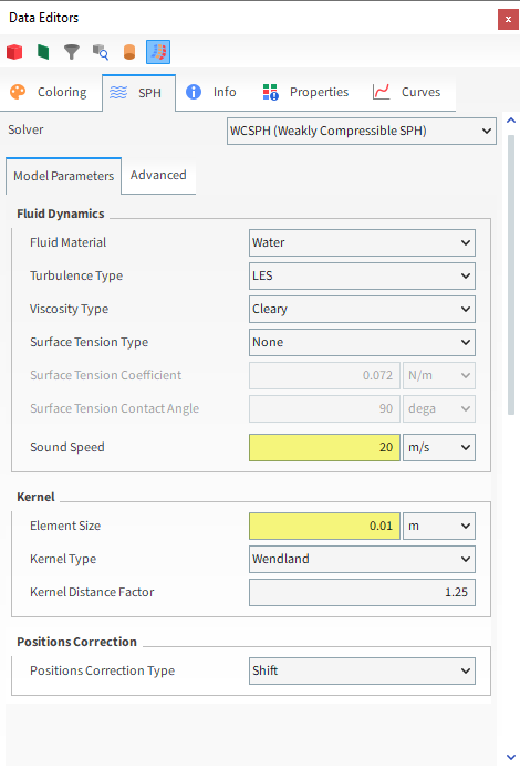
Tip: Refer to the User Manual for more information about Sound Speed. For this tutorial, we change the default value by a reasonable value in order to have consistent results and reduce the simulation time.
With a 3D View opened, set your preference color for the fluid (SPH elements) from the Coloring tab on Node color section.
The Inlets and Outlets step enables you to create two kinds of inlets for fluids:
The Volumetric Inlet, that works for Fluid in the same way that it does for particles.
The Fluid Inlet, that injects fluid at a constant rate through an associated Geometry at a defined Time.
For this tutorial, we will create a Volumetric Inlet to fill part of the container with Water.
Follow the steps in the table below in order to create and define the inlet.
Step Data Entity Editors Location Parameter or Action Settings A Inlets and Outlets Create Volumetric Inlet B Inlets and Outlets ﹂Volumetric Inlet <01>
Volumetric Inlet Name Water Fill Volumetric Inlet | SPH Mass 800 [kg] … | Region Seed Coordinates 0.2, 0.15, 0.305 [m] Box Bounds | Center Coordinates 0.2, 0.15, 0.305 [m] … | Dimensions 0.4, 0.3, 0.61 [m]
In a 3D View it is possible to visualize the region to be filled when Water Fill Inlet is selected.
Note: You can also set the dimensions and center of the region with the mouse by clicking and dragging the slider handles attached to each face or to the center of the cubic region (for this tutorial, please keep the values you just defined).
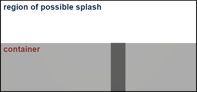
For the Domain Settings step, we will define a custom boundary box that exceeds the limits of our wall geometries.
Doing this will allow Rocky to compute the elements that possibly escape above the container region (splash from the collision with the column or container).
By default Rocky automatically creates a Domain box based upon the boundary limits of the Walls.
Any element that leaves those limits is eliminated from the simulation.
These default settings would not work for the dam break simulation as the water splashes over the container region.
Use the information in the table that follows to set the Domain and Solver.
Step Data Entity Editors Location Parameter or Action Settings A Domain Settings Domain Settings Use Boundary Limits (Cleared) Min Values 0, 0, 0 [m] Max Values 1.6, 0.75, 0.61 [m] B Solver Solver | Time Simulation Duration 3.5 [s] Output Settings | Time Interval 0.01 [s] Solver | General Simulation Target GPU ⯆
Note: The GPU is preferred in this case, but the simulation can also be run with a CPU.
You can check the resulting Domain in a 3D View.
Keep in mind that the Solver | Output Properties tab allows you to select which Properties data will be saved in disk for post-processing. This allows for faster processing and lower storage footprint by disabling Properties that you are not interested in analyzing. The entities from which you may enable or disable data collection are:
CFD
Contacts
Geometries
Joints
Particles
SPH
From the Modules Properties tab, you may also select which Properties that are allowed by Modules you want to keep.
Note: External Modules might make new Properties available for different simulation entities, not necessarily restricted to the Modules Properties tab.
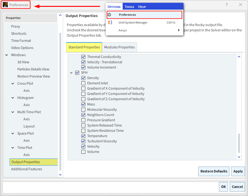
In this version of Rocky, not all SPH Properties are enabled by default. You may enable/disable the SPH Properties you want from the Output Properties tab in the Solver Data Editors panel.
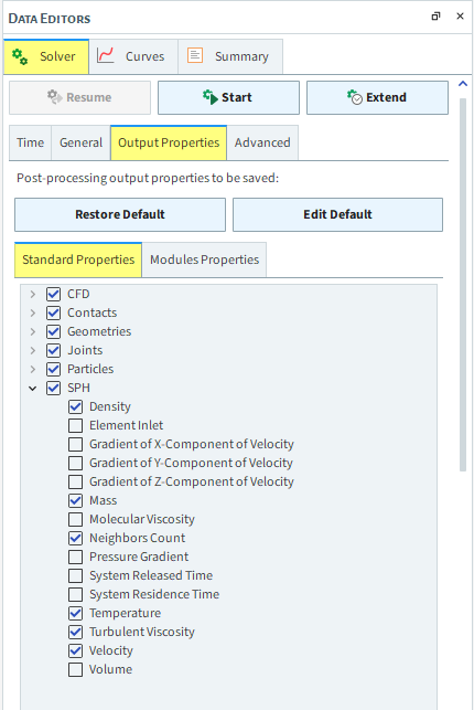
In case you wish to have some or all SPH Properties enabled in your future simulation projects, you can also have them enabled by default. From Options in the Rocky Menu, select Preferences and navigate to Output Properties. From the Output Properties window, you can select which SPH Properties you want enabled or disabled by default in your Rocky projects.
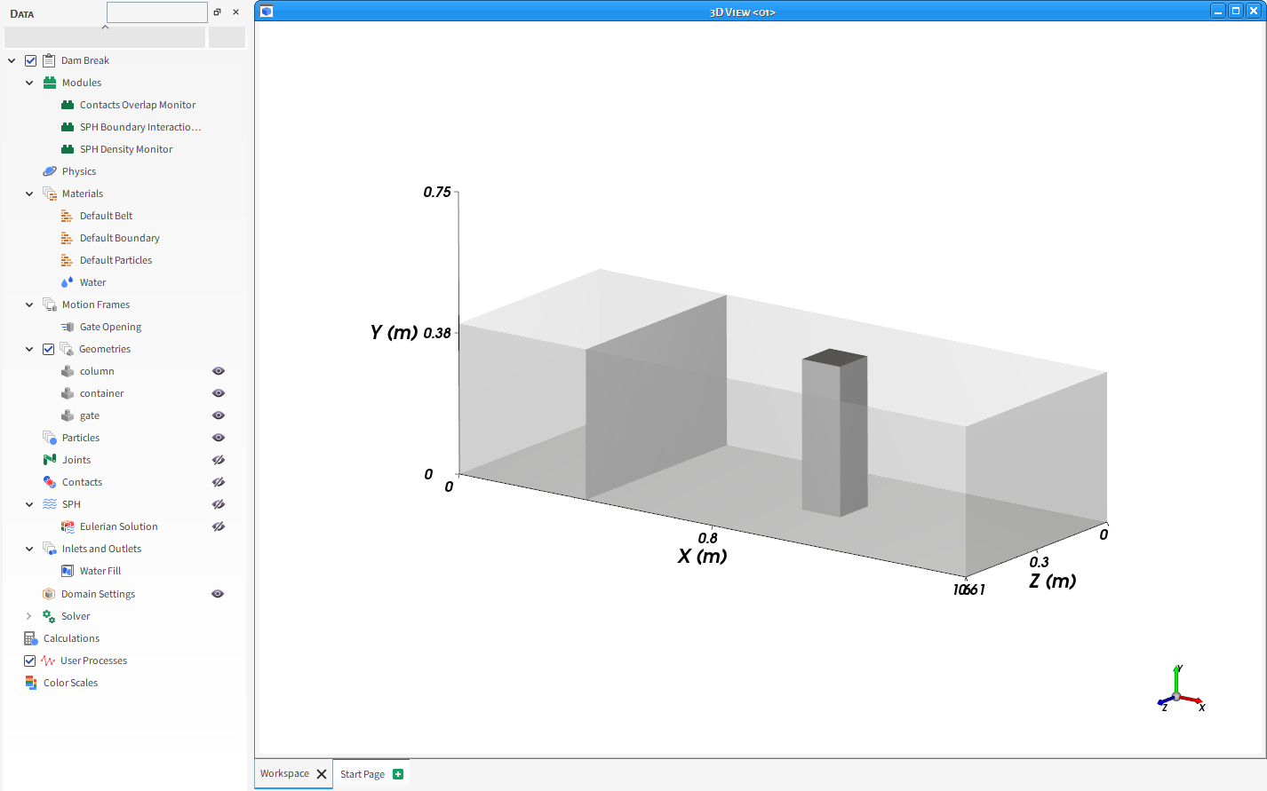
With a 3D View opened, your Data panel and Workspace should look similar to the below image.
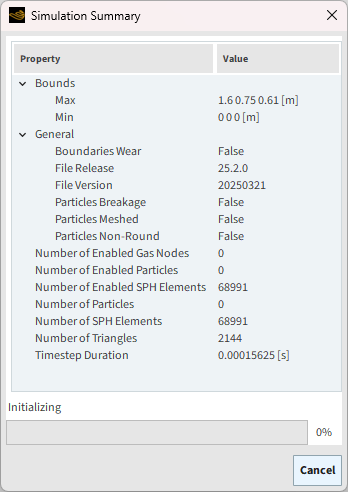
From the Solver entity, click Start.
The Simulation Summary appears, then processing begins.
This completes Part A of this tutorial, in which Rocky was used to set up and process a Dam Break simulation.
During this tutorial, it was possible to:
Enable a Module.
Define a Fluid and a Fluid Inlet.
Visualize SPH parameters.
Define a Domain.
What's Next?
If you completed this tutorial successfully, then you are ready to move on to Part B and post-process this project.
The purpose of this tutorial is to analyze a fluid (SPH) simulation after you have processed it. We will continue from where we left off in Part A.
You will learn how to:
Create a fluid surface
Visualize SPH Properties in a 3D View Window
Analyze the Eulerian Solution
And you will use these features:
Animation panel
Eulerian Solution
Time plot
User Process - Cube
User Process - Plane
If you completed Part A of this tutorial, ensure that Rocky project is open. (Part B will continue from where Part A left off.)
If you did not complete Part A, do all of the following:
Download the
dem_tut24_files.zipfile here .Unzip
dem_tut24_files.zipto your working directory.Open Rocky 2025 R2.
Important: To make use of the Rocky project file provided, you must have Rocky 2025 R2 or later. If you have an earlier version of Rocky, please upgrade to the latest version, or complete Part A from scratch.
From the Rocky program, click the Open Project button, find the
dem_tut24_filesfolder, and then from thetutorial_24_A_pre-processingfolder, open thetutorial_24_pre-processing.rockyfile.Process the simulation. (From the Simulation toolbar, click the Start button.)
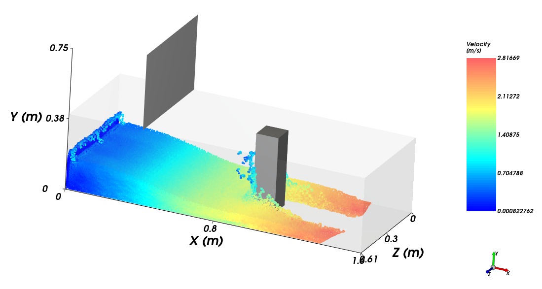
Let's start by coloring our fluid elements by velocity.
From the Data panel, select SPH and then from the Data Editors panel, select the Properties tab.
Select Velocity and then drag and drop it onto the 3D View window.
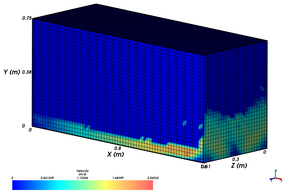
To represent SPH data as continuous fluid, let's use the Eulerian Solution to continue the post-processing.
We will first color the cells by Velocity, in order to compare the results we had by coloring the SPH elements.
From the Data panel, on the SPH field, select Eulerian Solution and then from the Data Editors panel, select the Coloring tab.
Expand Faces and then select Velocity from the drop down list as Property.
Use the eye icons to make Eulerian Solution visible and hide everything else but the Velocity color scale.
Note: You will view only data from the most external cells from the domain. To see results from an specific area, you can create a cube, cylinder or a plane User Process from the Eulerian Solution entity and follow the same procedure.
In this tutorial, we are interested in analyzing the region where Water collides with the column (middle of the container).
We will create a Plane in order to visualize this region with the Eulerian Solution (continuous data).
Let's also create a Cube to see the elements in this region with the SPH (discrete) entity.
Follow the steps in the table below to create both User Processes.
Step Item Location Parameter or Action Settings A Eulerian Solution Create a Plane User Process B User Processes ﹂Plane <01>
Plane Angle 90 [dega Plane Normal 0, 1, 0 [ - ] Coloring Edges (Cleared) Faces | Property Velocity ⯆ C Windows (Panel) Create a new 3D View D SPH Create a Cube User Process E User Processes ﹂Cube <01>
Cube Center 0.8, 0.38, 0.305 [m] Magnitude 1.6, 0.75, 0.02 [m] Coloring Nodes (Enabled) Nodes | Property Velocity ⯆
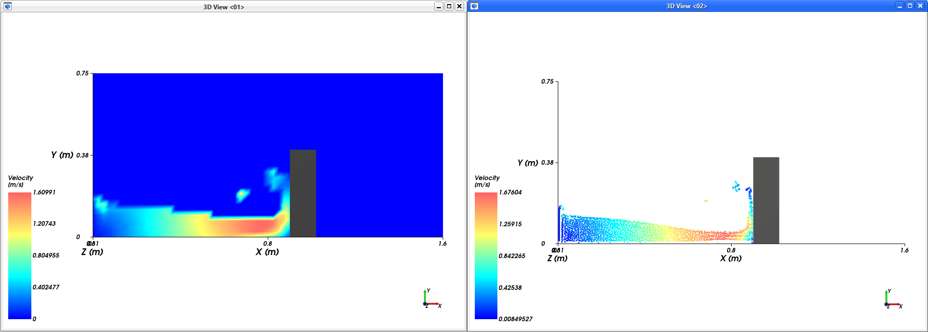
Finally, let's visualize and compare the fluid views between SPH (discrete) and Eulerian Solution (continuous) data.
From the Windows panel, select the 3D View <01> and use the eye icons to hide everything but the Plane <01>, column and Velocity color scale.
Select the (recently created) 3D View <02> and use the eye icons to hide everything but the Cube <01>, column and Velocity color scale.
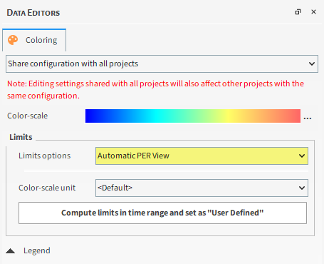
On the Data panel, from Color Scales, select Velocity, and from the Data Editors panel, ensure Limits options is defined as Automatic PER View.
Use the mouse to adjust the views in a way you can compare them (as shown).
Tip: If you are using a full screen in the workspace, use the button located on the upper right in order to make the window adjustable.
Use the slider from the time bar to choose the timestep you want to analyze.
We will also make use of a Filter User Process in order to visualize a fluid surface.
To represent it, we will restrict Eulerian Solution data based upon a value for a property defined as Weight.
The value of the properties (velocity, density, etc.) for each node of the interpolation grid is based on an interpolation, using the kernel function*, of the values of the SPH elements inside the kernel radius.
The Weight property gives the summation of the weight of all SPH elements that affect each grid node.
This property can be used to define the fluid surface as it is related to the concentration of SPH elements around the nodes.
If the region has no SPH elements, the Weight returns 0.
When the region is full of elements, the function tends to return a value close to 1.
* Refer to SPH Technical Manual to learn more about SPH Kernel functions.
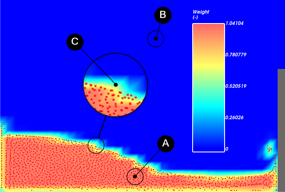
To better understand how the Weight is calculated, see the images below.
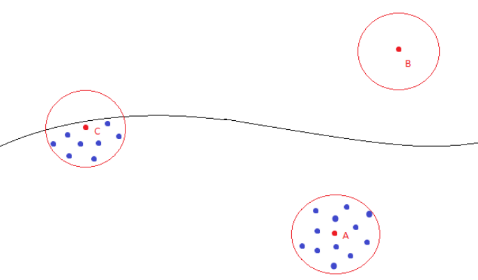
Point A: Weight (approximately) 1
Point B: Weight = 0
Point C: 0 < Weight < 1
As the volume around C is half empty, half full of elements, Weight tends to return 0.5. (see the Color Scale in the reproduced scheme into Rocky below)
Follow the steps in the table below to create a weight based isosurface.
Step Data Entity Editors Location Parameter or Action Settings A Eulerian Solution Create a Filter User Process B User Processes ﹂Filter <01>
Property Name Water Surface Property Weight ⯆ Mode Cut ⯆ Cut Value 0.5 [ - ] Coloring Transparency (Enabled) Faces | Property Velocity ⯆ Edges (Cleared)
Tip: Ensure that Faces checkbox is enabled and the other ones are disabled for Property <01> | Coloring.
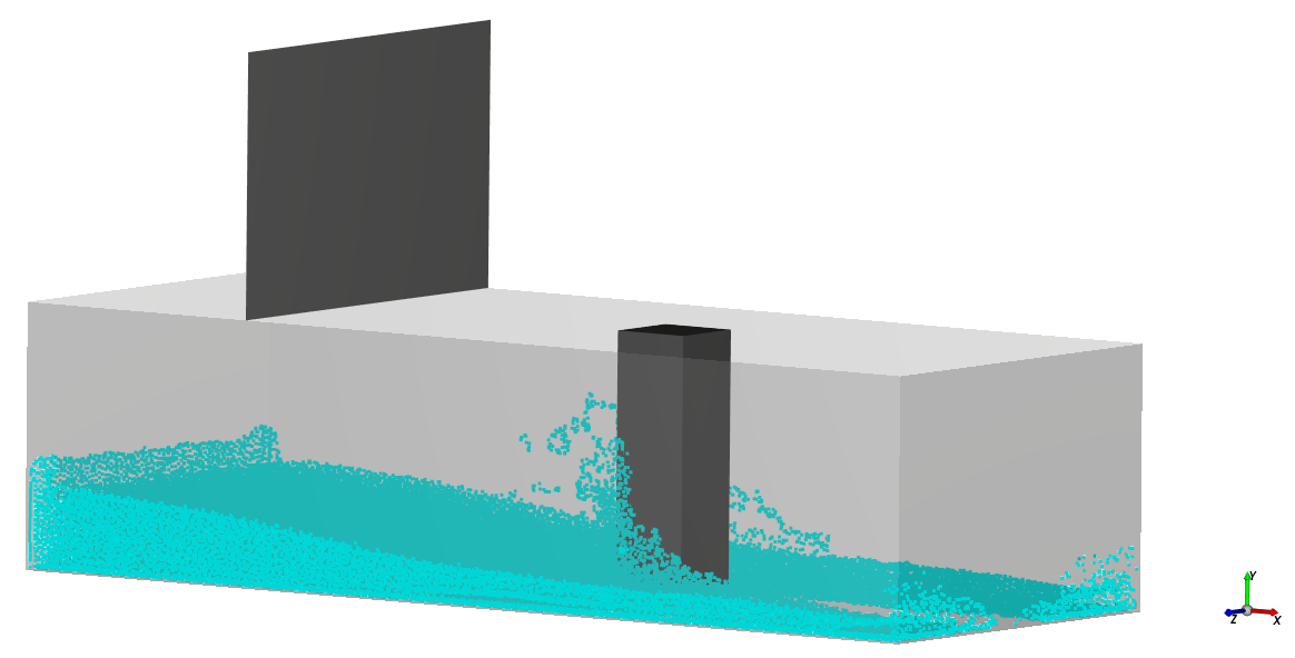
You can visualize the resulting surface for all timesteps in a 3D View. 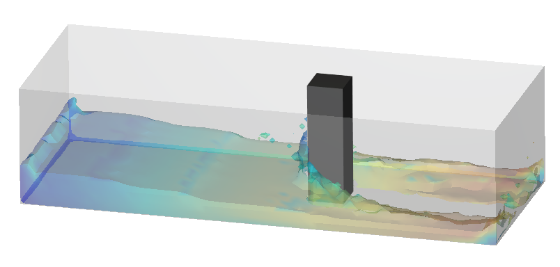
Let's create an animation to visualize the fluid behavior with the created surface.
Tip: Hide everything but the Geometries and Water Surface.
Follow the steps in the table below to create a video of your simulation.
Step Item Parameter or Action Settings A Tools (menu) Enable Animation Panel B Animation FPS 100 [ - ] Time (0s) Add Key Frame (button) Frame | Number of Frames 350 [ - ] Time (3.5s) Add Key Frame (button) Click the Play button to preview it, and the Export Animation button to save the movie to an AVI file.
In a dam break simulation, the magnitude of fluid forces in wall geometries is a result of interest.
In this tutorial we will analyze the resulting fluid force in the column in the X (fluid flow) direction for all timesteps.
We will also visualize the maximum fluid force in a column triangle in order to see where it occurs in the wall.
Follow the steps in the table below to create a Time Plot with both force values .
Step Data Entity Editors Location Parameter or Action Settings A Geometries ﹂column
Curves SPH : Force : X Show curve in new Plot Properties SPH : Force : Nodal : X Show in selected Time Plot by Max
The resulting plot is shown below.
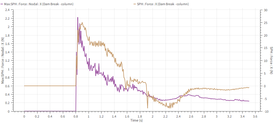
Note: Press Shift+Click over a curve point to inspect its values.
By inspecting the plot values, it is possible to see that the maximum force value in a column triangle occurs at 0.83 s.
Note: Your results may differ slightly from the ones presented in this tutorial.
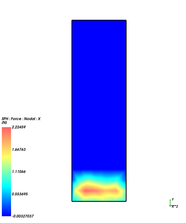
Follow the table to color the column by nodal forces in a 3D View in order to visualize the region of the wall that the force is occurring.
Step Data Entity Editors Location Parameter or Action Settings A Geometries ﹂column
Coloring Transparency (Disabled) Faces (Enabled) Faces | Property SPH : Force : Nodal : X ⯆ With a 3D View opened, from the Time Toolbar, select the time that the maximum force occurs (in this tutorial, 0.83 s).
You can visualize the point where the maximum fluid force occurs in the 3D View by hiding everything but the column and the SPH : Force : Nodal : X Color Scale.
Note: The maximum force occurs when the water first collides with the column, in the base of the column. You can use the shortcut Shift+X to see the face in a normal view.
This completes Part B of this tutorial.
Rocky was used to analyze a dam break.
During this tutorial, it was possible to:
Set up a fluid-only simulation
Visualize Properties in a 3D View window
Use post-processing tools to filter data and visualize water surface
Create an animation of a SPH simulation
Plot Curves and Properties