


(Part A) Set up a CFD case with heat transfer in Ansys Fluent to be later used in a two-way coupling simulation with Rocky DEM.
(Part B) Use the CAS file you created in Part A to set up the Rocky portion of the two-way simulation, and then run it coupled with Ansys Fluent.
(Part C) Post-process in Rocky the 2-Way Fluent coupling simulation you completed in Part B.
The main purpose of this Tutorial is to set up a CFD case with heat transfer in Ansys Fluent to be later used in a two-way coupling simulation with Rocky DEM.
Important: Even if you are already familiar with CFD, please follow Part A in order to understand the main limitations and needs for single-phase coupling with Rocky.
Part B and Part C of this tutorial will cover setting up the Rocky project and running the two-way coupled simulation, respectively.
The scenario being used in this tutorial includes a bed of initially hot particles being fluidized in a colder air current.
Fluidized beds are widely adopted in the chemical industry due to the enhanced mixing and improved heat and mass transfer between the particles and fluid.
You will learn how to: Set up and save a single-phase heat transfer case in Ansys Fluent that can later be used for two-way coupling with Rocky DEM.
To complete this tutorial, you are required to have a valid license for Ansys Fluent and Rocky 2025 R2.
Important: This ADVANCED tutorial assumes that you are already familiar with the Ansys Fluent UI and project workflow.
If that is not the case, please refer to the Ansys Fluent user documentation for basic introduction about Fluent usage before beginning this tutorial.

The walled rectangular container used in this tutorial is composed of the following geometries:
(1) walls, which itself contains two additional components:
(a) inlet
(b) outlet
Note: These three geometries will come from the Fluent .cas file that you will set up as part of this tutorial.
To set up the Fluent Case, do the following:
Open Ansys Fluent.
From the Fluent Launcher, under Dimension, ensure that 3D is selected; also, under Options, ensure that Double Precision is selected (as shown).
Important: Double Precision and 3D are required for coupling with Rocky.

Click Start.
For this tutorial, we will start by importing a mesh file.
Download the
dem_tut14_files.zipfile here .Unzip
dem_tut14_files.zipto your working directory.From the File menu, point to Read, and then click Mesh.
From the Select File dialog, do the following:
From the Files of type list, select All Mesh Files (*.msh* *.MSH*).
From the dem_tut14_files/mesh folder, select the tutorial_14_mesh.msh file, and then click OK.
Now that the Fluent .msh file is imported, we can start setting up the Fluent case.
Use the information in the table that follows to visualize and set up the mesh.
Tip: If you run into settings or procedures in these tables that you are not yet familiar with, please refer to your Ansys Documentation to find detailed instructions.
Step Item Location Parameter or Action Settings A Setup ﹂General
Task Page Display Mesh (inlet, outlet, walls | Display) Check Mesh Time Transient Gravity (Enabled) Gravitational Acceleration -9.81 [m/s2] in the Z direction Important: Transient must be selected in order to run a two-way coupled simulation.
In this tutorial, we will be setting up the Fluent case with only one fluid phase (air).
This single phase approach is:
Faster than the equivalent simulation using multiple phases.
Easier to set up and allows for a broader range of models.
Tip: Since this tutorial refers only to the single phase approach, refer to the Rocky CFD Coupling Technical Manual for information about using the multiphase approach.
(From the Rocky Help menu, point to Manuals, and then click CFD Coupling Technical Manual.)
From the Outline View, under Models, leave the Multiphase model Off (no changes).
For this tutorial, we want to enable both heat transfer and turbulence.
Use the information in the table that follows to continue setting up your case.
Step Item Location Parameter or Action Settings A Setup ﹂Models
﹂﹂Energy
Energy (dialog box) Energy Equation (Enabled) B Setup ﹂Models
﹂﹂Viscous
Viscous Model (dialog box) Model k-epsilon (2-eqn) Near-Wall Treatment Scalable Wall Functions Note: The choice of turbulence model depends upon the application.
For the Materials properties, we will be using the default Fluid properties for air.
For the Boundary Conditions properties, we will use the default (adiabatic) properties for Wall, but we will define new conditions for the Inlet and Outlet.
Use the information in the table below to continue setting up your case.
Step Item Location Parameter or Action Settings A Setup ﹂Boundary Conditions
﹂﹂Inlet
Velocity Inlet (dialog box) | Momentum Velocity Magnitude 2 [m/s] Turbulence | Specification Method Intensity and Hydraulic Diameter ⯆ Turbulence | Hydraulic Diameter 0.1 [m] Velocity Inlet (dialog box) |Thermal Temperature 293.15 [K] B Setup ﹂Boundary Conditions
﹂﹂Outlet
Pressure Outlet (dialog box) | Thermal Backflow Total Temperature 293.15 [K]
Use the information in the table that follows to define the solution methods.
Step Item Location Parameter or Action Settings A Solution ﹂Methods
Task Page Pressure-Velocity Coupling | Scheme SIMPLE Transient Formulation First Order Implicit Note: With the single phase approach, there is no limitation on which pressure-velocity coupling scheme you can use.
In addition, for all two-way coupling simulations, First Order Implicit must be set for Transient Formulation.
Use the information in the table that follows to initialize and set the calculation parameters.
Step Item Location Parameter or Action Settings A Solution ﹂Initialization
Task Page Initialization Methods Standard Initialization Compute from all-zones ⯆ Initialize B Solution ﹂Run Calculation
Task Page Time Advancement | Type Fixed ⯆ Time Step Size 0.001 [s] Important: To run a coupled simulation, the Time Advancement | Type must remain Fixed.
Because this is a two-way coupled simulation, we will not be solving the CFD case at this point but will be saving this setup to a .cas file that will be connected with Rocky later.
Save the case by doing the following:
From the File menu, point to Write and then click Case.
From the Select File dialog, do all of the following:
Choose a folder location.
Enter the Case File name as fluidized_bed.cas.h5.
Click OK.
This concludes Part A of this tutorial.
For further information on the topic presented, we suggest searching the CFD Coupling Technical Manual, which provides descriptions of the DEM-CFD coupling methods.
To access it, from the Rocky Help menu, point to Manuals, and then click CFD Coupling Technical Manual.

For further information about Ansys Fluent, please refer to the Ansys Fluent user documentation.
Ansys Fluent was used to set up a single-phase CFD simulation with heat transfer that will later be used for two-way coupling with Rocky.
During this tutorial, it was possible to:
Use Ansys Fluent to set up a single-phase CFD case
Save the case file for later two-way coupling with Rocky
What's Next?
If you completed this tutorial successfully, then you are ready to move on to Part B and create the Rocky project that will later be coupled with this CFD case.
The main purpose of this Tutorial is to use the .cas file we created in Part A to set up the Rocky portion of the two-way simulation, and then run it coupled with Ansys Fluent.
As a reminder, the scenario covered includes a bed of initially hot particles that are fluidized in a colder air flow.
You will learn how to:
Import geometry components from a Fluent .cas file
Set up and save a fluidized bed simulation with Rocky
Save a Rocky project for restart
Set up and run a 2-Way Fluent coupled simulation in Rocky
And you will use these features:
Thermal Model
Custom Geometry Import
2-Way Fluent CFD Coupling
To complete this tutorial, you are required to have a valid license for Ansys Fluent and Rocky 2025 R2.
Important: This ADVANCED tutorial assumes that you are already familiar with the following programs and resources:
The Rocky program.
If this is not the case, it is recommended that you complete at least Tutorials 01- 05 before beginning this tutorial.
The Ansys Fluent program.
If this is not the case, please refer to the Ansys Fluent user documentation for a basic introduction about Fluent usage before beginning this tutorial.

As a reminder, the walled rectangular container used in this tutorial is composed of the following geometries:
(1) walls, which itself contains two additional components:
(a) inlet
(b) outlet
Note: These three geometries will come from the Fluent .cas file that you will import into Rocky.
Do one of the following:
If you completed Part A of this tutorial, ensure you have available the fluidized_bed.cas.h5 file you created in Fluent. (Part B will make use of that file.)
If you did not complete the project from Part A, ensure you have downloaded and extracted the
dem_tut14_files.zipfile here .
Open Rocky 2025 R2.
Create a new project.
Save the empty project to a location of your choosing.
Use the information in the tables that follow to start setting up your Rocky project.
Tip: If you run into settings or procedures in these tables that you are not yet familiar with, please refer to the Rocky User Manual and/or other Tutorials (via the Introductory Tutorials and Advanced Tutorials) to find the detailed instructions you need.
Step Data Entity Editors Location Parameter or Action Settings A Study Study Study Name Fluidized Bed B Physics Gravity Y-direction 0 [m/s2] Z-direction -9.81 [m/s2] Momentum Numerical Softening Factor 0.1 [ - ] Thermal Enable Thermal (Enabled) Conduction Correction Model Morris et al. Area+Time ⯆ C Geometries Import Wall fluidized_bed.cas.h5 with "m" for Import Unit D Geometries ﹂walls
Wall | Thermal Thermal Boundary Type Adiabatic E Materials ﹂Default Particles
Material Use Bulk Density (Cleared) Density 1500 [kg/m3] Young's Modulus 1e+07 [N/m2] Thermal Conductivity 1.4 [W/m.K] Specific Heat 800 [J/kg.K] F Particles Create Particle G Particles ﹂Particle <01>
Particles Name smaller Particles | Size Size 0.003 [m] @ 100% H Particles Create Particle I Particles ﹂Particle <01>
Particles Name bigger Particles | Size Size 0.005 [m] @ 100% Note: The walls may be already set as Adiabatic for Step D.

Next, we will create a Volumetric Inlet and will constrain it to achieve a flat pile.
Where you place your Seed Coordinate and how you constrain your fill affects the behavior of particles after release. For example, when constraining by Geometries:
(1) A Seed Coordinate placed too high above the geometry base might cause particles to fall.
(2) To achieve a more settled pile, locate your Seed Coordinate closer to the base of the geometry (but avoid the very bottom).
(3) Choosing to Use Geometries to Compute the Box bounds could result in a rounded pile.
(4) To achieve a flat pile, define your own Box bounds.
Use the information in the table that follows to continue setting up your Rocky project.
Step Data Entity Editors Location Parameter or Action Settings A Inlets and Outlets Create Volumetric Inlet B Inputs ﹂Volumetric Inlet <01>
Volumetric Inlet | Particles Add 2 entry rows (1) Particle | Mass | Temperature smaller ⯆ @ 0.06 [kg] & 363 [K] (2) Particle | Mass | Temperature bigger ⯆ @ 0.06 [kg] & 363 [K] Volumetric Inlet | Region Seed Coordinates 0, 0, 0.01 [m] Geometries (All Enabled ("Check All")) Box bounds | Center Coordinates 0, 0, 0.025 [m] Box bounds | Dimensions 0.1, 0.1, 0.1 [m]

Tip: From a 3D View window, you can visualize the Seed Coordinate (blue dot) and the Box bounds (blue cube) that will constrain your Volumetric Inlet.
Important: The Seed Coordinate must be located within your Box Bounds.
You can change the location and dimensions of the bounding box from within the 3D View window by clicking and dragging the handles (colored dots) representing the center, and the local X, Y, and Z locations respectively.
You must still move the Seed location by using only the Seed Coordinates values.
For this tutorial, keep the both the Box bounds and Seed Coordinates as defined previously.
Use the information in the table that follows to finish setting up your Rocky project.
Step Data Entity Editors Location Parameter or Action Settings A Solver Solver | Time Simulation Duration 0.1 [s] Output Settings | Time Interval 0.02 [s] Solver | General Simulation Target CPU ⯆
With a 3D View window opened, your Data panel and Workspace should look similar to the below image.

From the Solver entity, click Start.
The Simulation Summary screen appears (as shown), then processing begins.


Tip: You can use the Auto Refresh checkbox to view in a 3D View window the results during processing.
Once the simulation is done processing, do the following:
From the Coloring service toolbar, color the Particles by Velocity : Translational : Absolute (as shown).

From the Time toolbar, do all of the following:
Click the Play simulation button or use the Next timestep button to move through the simulation output times. You will see the particle pile settle (slightly) due to gravity.


Click the Pause simulation button, and then click the Last timestep button to go to the end of the simulation.
This will be the initial state of the particles when coupling with Fluent.
Now that the bed of particles is defined, save this simulation for Restart.
From the File menu, click Save project as...

From the Save As dialog, select the last option, Save as a New Project for Restart, and then click OK.

This will save the project (setup and current particle location information) at the timestep you have selected, which for this example, should be the last time step.
From the Save File dialog, select a location and File name for the new project, and then click Save.
The newly saved project should now have the same bed of particles with the timestep reset to zero.

This is the Rocky project with which we will now two-way couple with Fluent.
For the CFD Coupling step, we will select the 2-Way Fluent option.
This option in Rocky takes into account fluid forces acting on particles and transfers particle information back to Fluent.
From Study, click Enable CFD Coupling and select 2 -Way Fluent from the Coupling Mode list.

From the Select Fluent CAS file dialog, navigate to and select the same Fluent .cas file you used earlier to import geometries*, and then click Open.
* As a reminder, do one of the following:
If you completed Part A of this tutorial, navigate to and select the .cas file that you created in Part A (fluidized_bed.cas.h5).
If you did not complete Part A, navigate to the dem_tut14_files folder that you previously downloaded, find the Fluent folder, and then select the fluidized_bed.cas.h5 file.
Important: A mesh validation step will occur immediately after the .cas file import. This requires a valid Fluent license on the same machine upon which you are running the Rocky simulation.

From the Data panel under CFD Coupling, select the new 2-Way Fluent option.
From the Data Editors panel, on the main 2-Way Fluent tab, there are five sub-tabs:

Interactions: This is where the particle-fluid correlations are defined, and where you will set the turbulent dispersion force (if applied).
Coupling: This is where you set the Fluent calculation mapping method and sub-stepping options.
Zones and Interfaces: This is where you can define how fluid cell zones and interfaces are treated in the coupled calculations.
Fluent: This is where you set solver options for the Fluent portion of the coupled simulation.
Variables: This is where additional variables or data that Fluent will receive from Rocky are listed (if defined).
For this tutorial, we will define only the Interactions and Fluent tab options.
From the Data Editors panel, select Interactions sub-tab.
Under Particle, multi-select both Particle groups, and then define the Convective Heat Transfer Law.
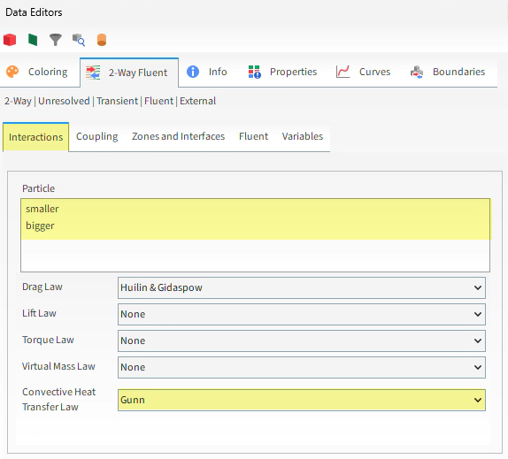
From the Data Editors panel, select the Fluent sub-tab, and then do all of the following:
From the Version list, select the Fluent version you want to use.
Clear the Keep all files checkbox (as shown). This allows you to save on disk space by choosing how many Fluent .dat files you want to keep.
Set the Files to keep option set to 2. This saves only the last two Fluent .dat files.

Tip: If you want to be able to post-process the CFD files in Fluent after processing, ensure that the Keep all files checkbox is enabled. (For this tutorial, however, keep the checkbox cleared.)
Use the information in the table that follows to set the Solver parameters for the coupled simulation.
Step Data Entity Editors Location Parameter or Action Settings A Solver Solver | Time Simulation Duration 3 [s] Solver | General Simulation Target CPU ⯆ Tip: If you have a GPU, you can use it for Rocky while Fluent uses the CPU processors.
From the Solver entity, click Start.
The Simulation Summary screen appears again.
In addition, Ansys Fluent will open automatically, and both Rocky and Fluent will begin processing your coupled simulation.
Tip: In Fluent, there is no need to refresh to see the results.
In Rocky, use the Refresh button or Auto Refresh checkbox to see the updated results in your 3D View window.

This concludes Part B of this tutorial.
For further information about setting up a Rocky project for coupling with Fluent, we suggest searching the Rocky User Manual.
For further information about setting up a Fluent case for coupling with Rocky, we suggest the following resources:
The webinar DEM and CFD Coupling
The Rocky CFD Coupling Technical Manual
The Fluent .cas file we created in Part A was used to set up the Rocky portion of the coupled simulation, and then we ran that Rocky simulation two-way coupled with the Ansys Fluent simulation.
During this tutorial, it was possible to:
Verify that Rocky has the components necessary to couple with Ansys
Import geometries from a Fluent .cas file into Rocky
Set up and Save for Restart a fluidized bed simulation in Rocky
Use Rocky to set up and run a two-way coupled simulation with Fluent
What's Next? If you completed this tutorial successfully, then you are ready to move on to Part C and post-process this project.
The main purpose of this Tutorial is to post-process in Rocky the two-way coupling simulation we completed in Part B.
As a reminder, the scenario covered includes a bed of initially hot particles that are fluidized in a colder air current.
You will learn how to:
Evaluate particle segregation
Analyze the mixing efficiency
Evaluate average particle temperature
Visualize fluid temperature
Analyze the pressure drop
And you will use these features:
User Processes, including:
Cube
Filter
Divisions Tagging Particle Calculations
Graphs and Plots, including:
Histograms
Time Plots
Table Time Plots
To complete this tutorial, you are required to have a valid license for Ansys Fluent and Rocky 2025 R2.
Important: This ADVANCED tutorial assumes that you are already familiar with the Rocky program.
If this is not the case, it is recommended that you complete at least Tutorials 01- 05 before beginning this tutorial.
If you completed Part B of this tutorial, ensure that Rocky project is open and has completed processing. (Part C will continue from where Part B left off.)
If you did not complete Part B, do all of the following:
Ensure you have a valid Fluent license on the same machine upon which you are running Rocky. (This is required in order to validate the mesh within the linked .cas file.)
Download the
dem_tut14_files.zipfile here .Unzip
dem_tut14_files.zipto your working directory.Open Rocky 2025 R2.
From the Rocky program, click the Open Project button, find the dem_tut14_files folder, and then from the tutorial_14_B_pre-processing-rocky folder, open the tutorial_14_B_pre-processing-rocky-restart.rocky file.
Process the simulation. (From the Data panel, select Solver and then from the Data Editors panel, click the Start button.)
Note: Ansys Fluent will open automatically, and both Rocky and Fluent will begin processing your coupled simulation.
Now that the project has completed processing, we can begin to analyze it.
Lets start by looking at particle segregation.
Use the information in the table below to begin this analysis.
Step Item Location Parameter or Action Settings A Window (menu) Create a New 3D View B Particles Coloring Nodes | Property Particle Group ⯆
Using the buttons on the Time toolbar, you can view how particles in the bed segregate as they are moved by the air injected from below.
Segregation: The bigger particles settle to the bottom while the smaller particles rise to the top of the bed.

We can also visualize how well particles in different regions of the container mix as the simulation progresses.
For this kind of analysis, we can use a Cube User Process along with Divisions Tagging to color the particles by the regional layers in which they were originally located.
To start this analysis, do all of the following:
From the Time toolbar, select the very first output time (0.00 s).
Use the information in the following table to create the Cube and Divisions Tagging processes.
Step Data Entity Editors Location Parameter or Action Settings A Particles Create a Cube User Process B User Processes ﹂Cube <01>
Cube Center 0, 0, 0.04 [m] Magnitude 0.1, 0.02, 0.08 [m] C Calculations | Particles Calculations Create a Division Tagging on <Cube 01> D Calculations ﹂Divisions Tagging (Cube <01>)...
Tagging Heigth Divisions 1 Depth Divisions 5 Coloring Faces | Property Divisions Tagging (Cube <01>)... ⯆ Particles inside the Cube have now been subdivided into 5 different axial divisions based on their position at t=0s.

Use the Data panel eye icons to hide Divisions Tagging(Cube <01>), hide Cube <01>, and show Particles.
From the Data panel, select Particles.
From the Data Editors panel, select the Coloring tab, and then under Nodes, select Divisions Tagging (Cube <01>) as the Property to be colored.

Notice how particles are distributed at the beginning of the simulation and advance in time to observe mixing.
Observe mixing: Based upon the particles' initial position (t=0), you can watch how they move around the bed as time advances.

Rather than looking at the entire bed as a whole, you can also focus your analysis on a single segment.
For this analysis, we will create another Cube in the middle of the bed and visualize how particles that originated from other segments are moved into that particular segment over time.
To start this new analysis, do all of the following:
From the Time toolbar, select the very first output time (0.00 s).
Use the information in the following table to create the Cube.
Step Data Entity Editors Location Parameter or Action Settings A Particles Create a Cube User Process B User Processes ﹂ Cube <02>
Cube Center 0, 0, 0.056 [m] Magnitude 0.1, 0.02, 0.0155 [m]
This new Cube should encompass the 4th axial division and should therefore contain only particles with Division Tagging equal to 4 at the beginning of the simulation.

Let's verify:
Use the information in the table that follows to create a histogram.
Step Item Parameter or Action Settings A User Processes ﹂Cube <02>
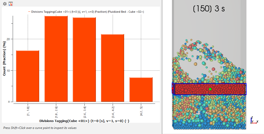
Show in new Histogram by Divisions Tagging (Cube <01>)... B Histogram (window) Configure histogram (button) C Configure Histogram (dialog box) Number of Bins 5 Percent Values (Enabled) Properties | Divisions Tagging (Cube <01>)... (Selected) Limits User Defined ⯆ Min 1 [ - ] Max 5 [ - ] The results (shown below) verify that at initial time (t=0), the 4th bin contains 100% of the particles.
Use the Time toolbar to advance the time and verify that particles coming from different initial positions move into this second cube, reducing the percentage of particles with tagging = 4.

Then, observe how particles are distributed at the final output time.

The results are shown below.
At the final output time (3 s), particles that originated from other divisions are more evenly distributed into the 4th axial segment of the bed.
Note: Your results may differ slightly from the ones presented in this tutorial.
You can also use a Filter User Process to further visualize and calculate the number of particles that enter and exit the segment of the bed we defined earlier (Cube <02>).
For this analysis, do all of the following:
From the Time toolbar, select the very first output time (0.00 s).
Use the table below to create the Property process and plot the results by particles mass.
Step Data Entity Editors Location Parameter or Action Settings A User Processes ﹂Cube <02>
Create a Filter User Process B User Processes ﹂Filter<01>
Property Property Divisions Tagging (Cube <01>) Cut Value 4 [ - ] C User Processes ﹂Cube <02>
Show in New Time Plot by Particle Mass D User Processes ﹂Filter <01>
Show in Current Time Plot by Particle Mass
The resulting plot shows the total mass of particles that have the divisions tagging equal to 4 inside the cube at each output time (blue), along with the total mass of particles inside the cube (orange).
At the start of fluidization, particles in section 4 were pushed out of their initial region, but moved back as time progressed and mixing continued.

Use the information in the table below to continue with this analysis.
Step Item Location Parameter or Action Settings A Time Plot <01> (window) Table (tab) Add Formula B Add Expression (dialog box) Curve Caption Tagging 4 mass fraction Curve Expression C/B This expression represents the ratio between the mass of particles that were initially in the 4th axial bin (Tagging = 4) and the current mass of particles inside that same bin area.
From the upper left corner of the Time Plot window, select the Plot tab.
The new curve (green) enables you to observe how the mass fraction of particles with Tagging 4 inside the Cube <02> has changed with time.

We can also analyze the Particles cooling down due to interactions with the fluid and container by plotting the Temperature property.
Use the information in the table to create the new plot.
Step Item Location Parameter or Action Settings A Window (menu) Create a New Time Plot B Particles Properties | Temperature Drag and drop onto the Time Plot window C Select The Statistics To Plot (dialog box) Min (Enabled) Max (Enabled) Average (Enabled) Right-click the grid, point to Axes Layout, and then select By Quantity.
In this plot, we can see how the average temperature of the particles decreases with time.

We can also visualize both the particle and fluid temperature in a 3D View window.
Use the table below to create this new view.
Step Item Location Parameter or Action Settings A Window (menu) Create a New 3D View B Fit (menu) Select Camera Preset: -Y C Geometries ﹂ walls
Coloring Transparency (Enabled) D Particles Coloring Nodes (Enabled) Nodes | Property Temperature ⯆
The temperature of the particles is shown.

Let's adjust the temperature scale to match the tutorial minimum and maximum limits, which are equal to the initial temperatures of the inlet (in Fluent) and particles (in Rocky), respectively.
Use the information in the table below to adjust the color scale.
Step Data Entity Editors Locations Parameter or Action Settings A Color Scales ﹂Temperature
Coloring Limit options User Defined ⯆ Limits 293.15, 363 [K] Color-scale unit degC ⯆ Continue defining the view by adding in the fluid temperature display.
Step Data Entity Editors Locations Parameter or Action Settings A CFD Coupling ﹂2-Way Fluent
Coloring Nodes (Enabled) Nodes | Property Fluid Temperature ⯆ Nodes | Point size 6 Follow the instructions for Step A to adjust the color-scale for Fluid Temperature so it matches the scale for particle Temperature.
The temperature of the fluid is shown along with the particles.

Tip: To better analyze the results, consider setting up both Color Scales with the same Limits and colors.
We can also calculate the pressure drop by using the fluid properties that come by default with 2-Way Fluent coupling.
To do this, we will create two Cubes one at the bottom of the container and another at the top and will calculate the difference in fluid pressure between the two locations.
Use the information in the table to create these two Cubes.
Step Data Entity Editors Location Parameter or Action Settings A CFD Coupling ﹂2-Way Fluent
Create a Cube User Process B User Process ﹂Cube <03>
Cube Name bottom Center 0, 0, 0.008 [m] Magnitude 0.1, 0.02, 0.0155 [m] C User Processes ﹂bottom
Create a Duplicate D User Processes ﹂bottom <01>
Cube Name top Center 0, 0, 0.492 [m]
You should now have two Cubes at each end of the container (as shown).

Now, lets plot the fluid pressure in both Cubes.
Use the information in the following table to create this plot.
Step Item Location Parameter or Action Settings A User Processes ﹂top
Properties | Static Presure Show in New Time Plot by Average B User Processes ﹂bottom
Properties | Static Pressure Show in Selected Time Plot by Average C Time Plot <03> (window) Table (tab) Add Formula D Add Expression (dialog box) Curve Caption Pressure Drop Curve Expression C-B Select the Plot tab.
In the plot, right-click the grid area, point to Axes Layout, and then select By Quantity.
At the top of the plot, click both Average data lines to turn off their displays (as shown).

The results show that after ~1 s, the system reaches a stabilized state. This period of time can be used to estimate an average pressure drop.
We can also post-process fluid information with Eulerian Statistics.
It is possible to calculate instantaneous or time-averaged fluid statistics based on the CFD cells located inside of each block from the eulerian division.
A property that can be analyzed within the divisions is the Solid Volume Fraction, that is the ratio between the summation of the particle volumes within a CFD cell and the volume of the cell.
Open a 3D View and use the information in the following table to analyze the instantaneous Solid Volume Fraction.
Step Item Location Parameter or Action Settings A CFD Coupling ﹂2-Way Fluent
Create a Cube User Process B User Processes ﹂Cube <03>
Create a Eulerian Statistics User Process C User Processes ﹂Eulerian Statistics <01>
Eulerian Statistics Heigth Divisions 3 Depth Divisions 20 Coloring | Faces Property Solid Volume Fraction ⯆ Show on Node? (Enabled) Hide the Particles entity and all the Geometries to visualize the Eulerian Statistics.
Click Shift+Y to see the instantaneous Solid Volume Fraction in the flow direction (as shown).

Take a moment and use the slider of the Time Toolbar to visualize the Solid Volume Fraction for different output times.
It is also interesting to visualize the fluid instantaneous velocity.
From the Coloring tab of the Eulerian Statistics <01> entity, define Property as Local Z-Velocity.
Use the slider bar from the Time Toolbar to see how the fluid velocity changes with the time.


This way you can get a continuous contour plot of the fluid velocity.
You can make Particles visible to see their influence on fluid behavior.
Note that the flow velocity is usually higher where particles are present due to the flow section area reduction.
Also note that the fluid gets decelerated by the particles due to energy dissipation.

Often we need to extract time averaged statistics instead of instantaneous information to compare against experimental data. This can be easily accomplished by using the Eulerian Statistics tool.
Use the table below to set up the time averaged fluid velocity.
Step Item Location Parameter or Action Settings A User Processes ﹂Eulerian Statistics <01>
Properties Add and edit time statistics properties (button) B Edit time statistics properties (dialog box) Add (button) C Add time statistics properties (dialog box) Start time 1 [s] Stop time 3 [s] Operations | Average (Enabled) Properties | Local Z-Velocity (Enabled) D User Processes ﹂Eulerian Statistics <01>
Coloring | Faces Property Average of Local Z-Velocity [1s, 3s]
Note: We choose a time interval that represents a steady state for the system to calculate the property average.

Note that, on average, the flow velocity is higher when passing through the particles area.
Also note that after passing through the particles, the average fluid velocity is almost the same for the rest of the bed.
This concludes Part C of this tutorial.
For more information about the tagging and divisions tagging tools, we recommend:
Reviewing the available post about Tagging and Divisions Tagging.
Searching the Rocky User Manual.
For more information about two-way coupling between Rocky and Ansys Fluent, refer to the CFD Coupling Technical Manual.
Rocky was used to post-process the Fluent Two-Way simulation that we ran in Part B.
During this tutorial, it was possible to:
Use the Particle Group property to analyze segregation.
Use User Processes and Divisions Tagging to analyze the mixing efficiency over time in discrete areas of the particle bed.
Plot the average Particle temperature as a function of Time.
Visualize both the particle and fluid temperature in a 3D View window.
Calculate the pressure drop using Cube User Processes and 2-Way Fluent Fluid Properties.
Visualize the fluid velocity profile in the air flow direction with Eulerian Statistics.
What's Next?
If you completed this tutorial successfully, then you are ready to move on to the next tutorial.