


In (Part A), you will create a Workbench project, and will set up and run a Rocky DEM simulation through Workbench.
In (Part B), you will couple the completed DEM simulation with Static Structural - Mechanical to calculate the FEA portion of the project. You will also use Workbench's Design Exploration feature to run additional simulations that optimize key project parameters.
The main purpose of this tutorial is to use Ansys Workbench to set up and run a DEM case in Rocky that will later be 1-way coupled with Ansys Static Structural - Mechanical.
Part B will cover 1-way coupling the DEM results with Static Structural - Mechanical to obtain the FEA results.
The scenario considered in this tutorial is that of a bin whose inadequate structure requires design modifications to better support its intended load.
You will learn how to:
Create a Workbench project and import a geometry
Connect the Workbench project to both Rocky and Ansys Static Structural - Mechanical
Open Rocky through Workbench
Ensure that Rocky is set up for FEA analysis
Refine the geometry mesh for optimal analysis
Define which load data to share with Mechanical
And you will use these features:
Ansys Workbench
(Rocky) Boundary Collision Statistics Module
(Rocky) External Coupling entity
To complete this tutorial, you are required to have a Windows machine, both of the following:
(1) A valid license for Ansys Mechanical 2025 R2, compatible with Transient Structural.
(2) A license of Rocky 2025 R2 or later.
Important: This ADVANCED tutorial assumes that you are already familiar the the following programs and resources:
The Rocky 2025 R2 program.
If this is not the case, it is recommended that you complete at least Tutorials 01- 05 before beginning this tutorial.
The Ansys Workbench platform.
If that is not the case, please refer to the Ansys Workbench user documentation for basic introduction about Workbench usage before beginning this tutorial.
Note: In this version of Ansys Rocky, the integration between Ansys Rocky and Ansys Workbench is automatically established during the installation process via Ansys Automated Installer. This also allows Forces to be automatically exported from Rocky to Workbench, without requiring manual export.
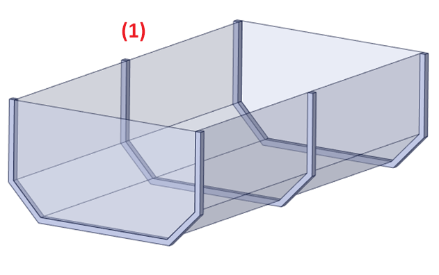
The geometry in this tutorial is composed of:
(1) Bin with supports
In the tutorial directory, the .dsco file for this geometry can be found.
Note: This geometry has been saved with the support components hidden as Rocky requires only the bin to interact with the particles.
To begin setting up the project, do the following:
Download the
dem_tut12_files.zipfile here .Unzip
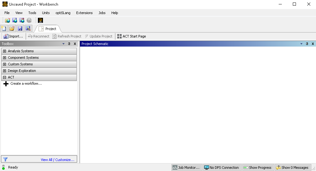
dem_tut12_files.zipto your working directory.Open Ansys Workbench 2025 R2.
Save the empty Workbench Project from the File, Save As... menu item.
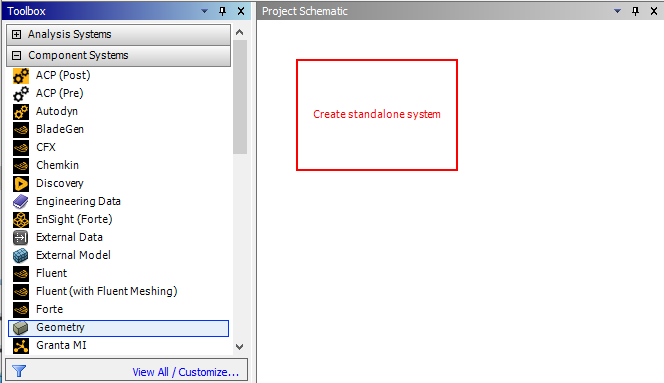
From the Toolbox panel, under the Component Systems item, drag and drop Geometry to the Project Schematic.
Right-click Geometry, point to Import Geometry, and then click Browse....

From the dialog that appears, locate the geometry folder inside dem_tut12_files you downloaded, select the input file Geometry.dsco, and then click Open.
Tip: The Geometry will show a green checkmark if the .dsco file is correctly imported.
From the Toolbox panel, under the Analysis Systems item, drag and drop Rocky onto the Geometry component of the Geometry block.
Note: Dropping the Rocky block onto the Geometry component will automatically generate a connection between the Geometry and Rocky.


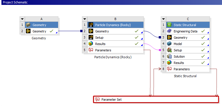
From the Toolbox, under Analysis Systems, drag and drop the Static Structural component onto the Results component of the Rocky block.

This creates an extra connection between the Results component on the Rocky block and the Model component on the Static Structural block that is not needed for this tutorial.
We must remove this extra connection otherwise Workbench will prevent us from opening Mechanical later (because it will be looking for Model information that does not exist).
Right-click the purple line connecting Results and Model, and then click Delete.

Save the Workbench project.
Tip: If you have only a single-instance Rocky license (typical for most users), ensure that the Rocky program is closed at this point.
In this next step, Workbench will open Rocky for you, and you will get errors if Rocky is already open.
From the Rocky block, right-click Setup, and then click Edit.

Note: While Rocky is processing, do not modify/save/close the connected Workbench session.
The Rocky interface opens automatically with the linked geometries already set up.

To start setting up your Rocky project, do the following:
From the Physics entity, on the Momentum tab, enable the Rolling Resistance Model of Type C: Linear Spring Rolling Limit.
For this tutorial, information about particle forces on the geometry will be used.
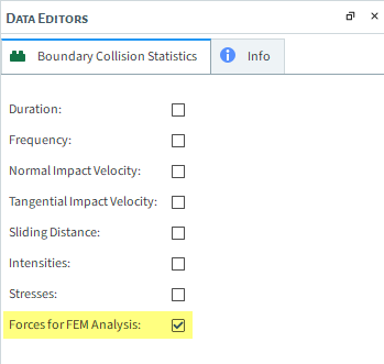
Enabling the collection of this data is accomplished through the Boundary Collision Statistics Module, by enabling the Forces for FEM Analysis checkbox.
Because the Rocky project is connected to Ansys Mechanical through Workbench, this collection is automatically enabled. However, to verify, do the following:
From the Data panel, under Modules, select Boundary Collision Statistics.
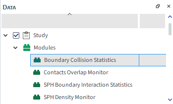
From the Data Editors panel, verify that the Forces for FEM Analysis checkbox is enabled.
For the Geometries step, you will notice that the geometries are automatically imported from the Geometry box in Workbench.
From the Data panel, under Geometries, select this already-imported surface item.
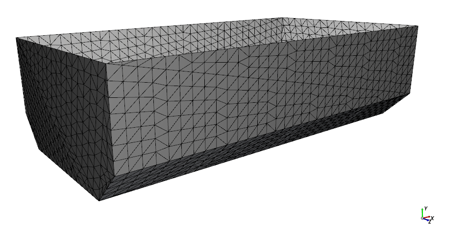
With a 3D View window open, visualize the meshing. (From the Data Editors panel, select the Coloring tab, and then enable the Edges checkbox.)

Since a coupled simulation with Ansys Mechanical will be carried out for this geometry part, it is important to refine the mesh so that the pressure field transferred to Mechanical has an adequate resolution for the desired structural analysis.
Every triangle node will provide a pressure vector, which will then be applied as a load inside Mechanical.
Refine the mesh as follows, then continue setting up your Rocky project:
From the Wall tab, on the Transform sub-tab, change the Triangle Size to 0.1 [m] (results shown).
Use the information in the table that follows to continue setting up your Rocky project.
Tip: If you run into settings or procedures in these tables that you are not yet familiar with, please refer to the Rocky User Manual and/or other Tutorials (via the Introductory Tutorials and Advanced Tutorials) to find the detailed instructions you need.
Step Data Entity Editors Location Parameter or Action Settings A Geometries Create Rectangular Surface B Geometries ﹂Rectangular Surface <01>
Rectangular Surface Center Coordinates 3.25, 3, 0 [m] Length 2.5 [m] Width 1.5 [m] C Particles Create Particle D Particles ﹂Particle <01>
Particle | Size (1) Size | Cumulative (%) 0.2 [m] @ 100% Particle | Movement Rolling Resistance 0.3 [ - ] E Inlets and Outlets Create Particle Inlet F Inputs ﹂Particle Inlet <01>
Particle Inlet Entry Point Rectangular Surface <01> Particle Inlet | Particles Add row (x1) (1) Particle | Mass Flow Rate Particle <01> @ 10000 [t/h] … | Time Stop 3 [s]

For this Tutorial, static loads on the bin geometry will be exported to Ansys Static Structural - Mechanical.
Because the loads are static, we need only to export the last output.
From the Data Panel, under External Coupling, select Wall Loads.
From the Data Editors panel, under Select Walls, select the surface checkbox, and then ensure the remaining options match the image below.

Use the information in the table that follows to continue setting up your Rocky project.
Step Data Entity Editors Location Parameter or Action Settings A Solver Solver | Time Simulation Duration 5 [s] Solver | General Simulation Target CPU ⯆
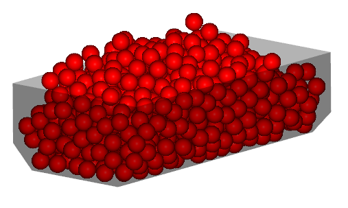
With a 3D View window opened, your Data panel and Workspace should look similar to the image shown.

From the Solver entity, click Start.
The Simulation Summary screen appears (as shown), then processing begins.

Tip: You can use the Auto Refresh checkbox to view in a 3D View window the results during processing.
Later in Part B of this tutorial, we will use the Force in the Y direction of the bin geometry to help determine whether modifications made during parameterization are improving the design.
We will expose this parameter to Workbench by making it available on the Output tab of the Expressions/Variables panel.
From the Data panel, under Geometries, select the surface geometry, and then from the Data Editors panel, select the Curves tab.
From the Tools menu, open the Expressions/Variables panel, and then select the Output tab.
From the Data Editors panel, select the Force : Y curve, and then drag and drop it onto the Output tab.

Select the newly added output, and then click the edit button.

From the Edit Properties dialog, define the values for Domain Range, and then click OK.

Your output should now be configured and ready to use (as shown).
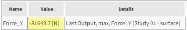
Note: Your results might differ slightly from those shown in this tutorial.
To complete this part of the tutorial, do the following:
Save your Rocky project.
Close Rocky.
Switch back to your Workbench project.
Note: Due to its connection with Workbench, nothing further is required in Rocky after processing is complete. There is no need to export any files. All necessary data transfers will happen in Workbench.
This completes Part A of this tutorial.
Through Ansys Workbench, we imported a bin geometry, set up the connection between Rocky and Ansys Static Structural - Mechanical, and set up and processed a simulation in Rocky that will later be 1-way coupled with Ansys Static Structural - Mechanical.
During this tutorial, it was possible to:
Verify that Rocky is ready for coupling with Ansys.
Create a new Ansys Workbench project, and import a geometry into Workbench.
Set up and run the Rocky portion of the simulation through Workbench.
Ensure the collection of forces data for later FEM analysis.
Expose several DEM parameters to Workbench for later analysis.
Define what geometry load data to later share with Mechanical.
What's Next? If you completed this part successfully, then you are ready to move on to Part B and set up and run the FEA simulation based upon these DEM results.
The main purposes of this tutorial are to use Ansys Workbench to run a 1-Way coupled DEM-FEA simulation using Rocky and Ansys Static Structural - Mechanical, and then optimize those results using Design Exploration.
We will make use of the Rocky DEM results we created in Part A.
As a reminder, the scenario considered in this tutorial is that of a bin whose inadequate structure requires design modifications to better support its intended load.
You will learn how to:
Use Workbench to transfer DEM results from Rocky to Static Structural - Mechanical
Set up and process the FEA simulation in Static Structural - Mechanical
Optimize key project parameters using Design Exploration
And you will use these programs:
Ansys Workbench, including Design Exploration
Ansys Static Structural - Mechanical
To complete this tutorial, you are required to have on a Windows machine, both of the following:
(1) A valid license for Ansys Mechanical 2025 R2, compatible with Transient Structural.
(2) A license of Rocky 2025 R2 or later.
Important: This ADVANCED tutorial assumes that you are already familiar the the following programs and resources:
The Ansys Workbench platform, including the Design Exploration functionality.
If that is not the case, please refer to the Ansys Workbench user documentation for basic introduction about Workbench and Design Exploration usage before beginning this tutorial.
The Ansys Static Structural - Mechanical program.
If this is not the case, please refer to the Ansys Mechanical user documentation for a basic introduction about Mechanical usage before beginning this tutorial.
If you completed Part A of this tutorial, ensure that the Ansys Workbench project you created is open. (Part B will continue from where Part A left off.)
If you did not complete Part A, do all of the following:
Download the
dem_tut12_files.zipfile here .Unzip
dem_tut12_files.zipto your working directory.Open Ansys Workbench.
Important: To make use of the Workbench project file provided, you must have Ansys 2025 R2 or later and Rocky 2025 R2 or later. If you have an earlier version of either of these programs, please upgrade to the latest version of Rocky and the latest version of Ansys that is supported by Rocky, or complete Part A from scratch.
From the Workbench program, click the Open Project button, find the dem_tut12_files folder, and then from the tutorial_12_A_processing-rocky folder, open the tutorial_12_A_processing-rocky.wbpj file.
With the project open in Workbench, you are now ready to begin Part B.
Before we set up the Mechanical project, we need to update the results:
From your Workbench project, on the Rocky block, right-click Results, and then click Update (as shown). Repeat this and click Refresh also.

This transfers the DEM results into Workbench, thereby making the data available to Mechanical.
Then, to initialize a static structural analysis using the DEM results:
From the Static Structural block, right-click Model, and then click Edit (as shown).

Ansys Mechanical opens with the linked geometry already included (shown on next screen).
Now, let's set up the Mechanical project.
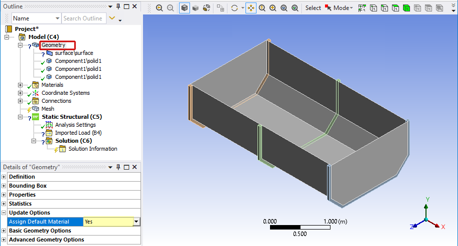
From the Outline panel, under Model, select Geometry.
In the Details of "Geometry" panel, under Update Options, define the Assign Default Material option.
From the Outline panel, under Model | Geometry, select surface\surface.
In the Details of "surface\surface" panel, under Definition, define the Thickness as 0.01 m and then click the box next to the Thickness label to create a parameter.
Under Properties, click the box next to the Mass label to create another parameter .
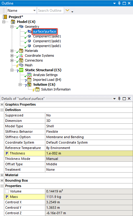
Note: The parameters we create here will later become outputs that we can use for design optimization in Workbench.
Create the first of two Named Selections by doing the following:
In the view, with the Face selection, multi-select the three lower faces of the support (as shown in red).
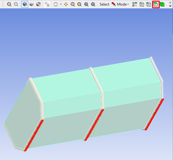
Right-click in the view, and then select Create Named Selection.
Define the Selection Name as "support".
Create the second of two Named Selections by doing the following:
In the view, with the Body selection, select the three support bodies (as shown in red).
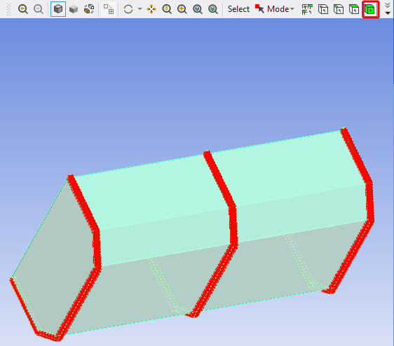
Right-click in the view, and then select Create Named Selection.
Define the Selection Name as "body-support".
Now, let's generate the mesh.
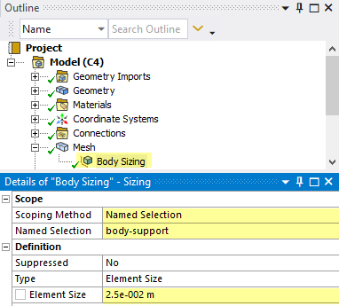
From the Outline panel, under Model, right-click Mesh, point to Insert, and then select Sizing.
Select the new Sizing entry, and then define the Scoping Method, Named Selection, and Element Size.
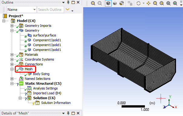
From the Outline panel, right-click Mesh, and then click Generate Mesh.
You can view the generated mesh by selecting Mesh from the Outline panel.
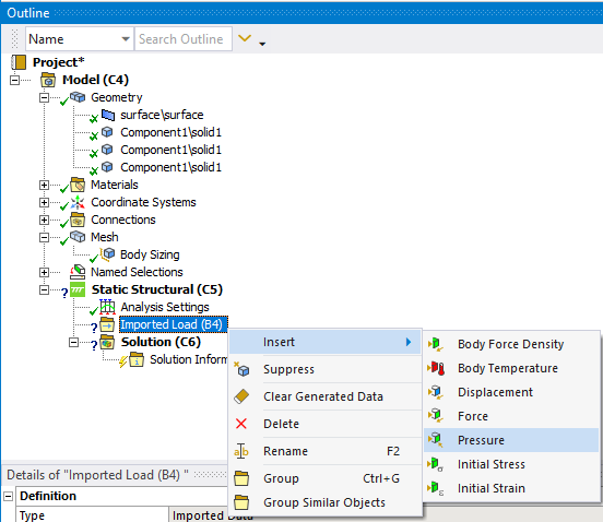
Define the imported pressure:
From the Outline panel, under Model | Static Structural, right-click Imported Load (B4), point to Insert, and then click Pressure.
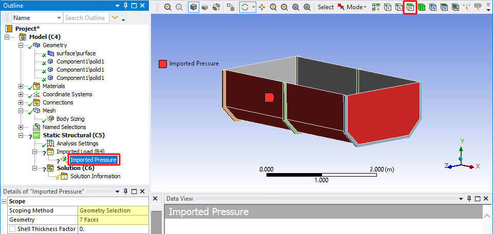
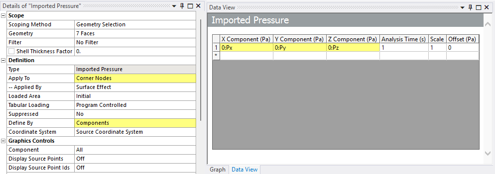
Select the newly added Imported Pressure entry.
From the Details of "Imported Pressure" section, under Scope, define the Scoping Method, and then using the Face selection, select all 7 faces of the bin.
From the Details of "Imported Pressure", select the Geometry field, and click Apply.
In the Definition section, define Apply To and Define By.
From the Data View window, define: X Component (Pa), Y Component (Pa), and Z Component (Pa) from the drop down lists (as shown).
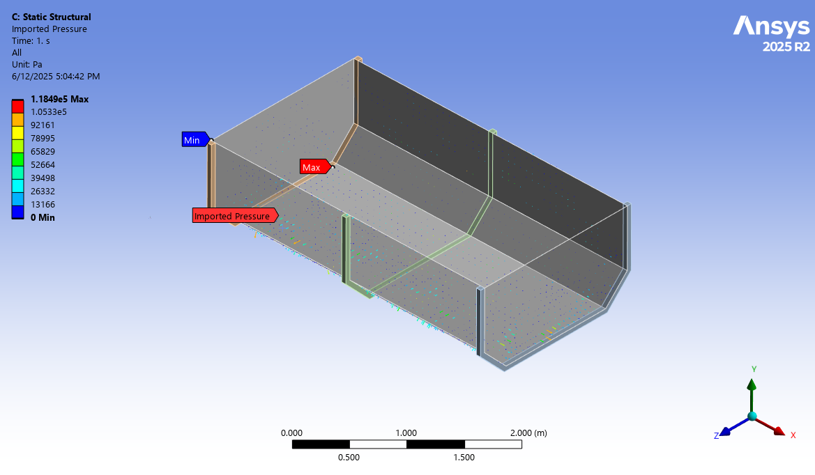
From the Outline panel, right-click Imported Pressure, and then select Import Load.
From the Outline panel, select Imported Pressure to show the vector plot of the imported load.
Next, define the fixed supports:
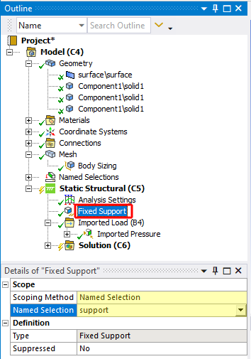
From the Outline panel, right-click Static Structural, point to Insert, and then click Fixed Support.
Select the new entry for Fixed Support.
From the Details of "Fixed Support" section, define the Scoping Method and Named Selection.
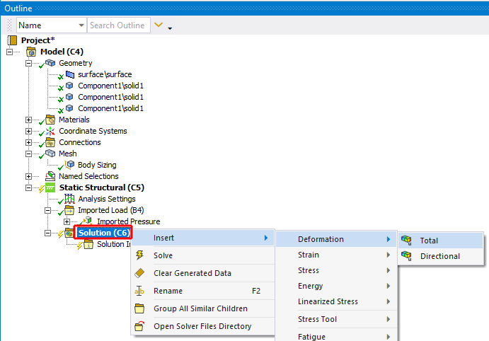
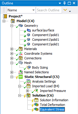
Now, let's define which solutions we want to analyze:
From the Outline panel, under Model | Static Structural, right-click Solution, point to Insert, point to Deformation, and then click Total (as shown).
Right-click Solution again, point to Insert, point to Stress, and then click Equivalent (von-Mises).
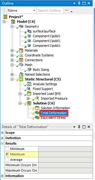
Select the newly added Total Deformation entry.
From the Details of "Total Deformation" panel, under Results, click the box next to the Maximum label to create a parameter.
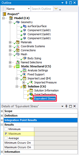
Repeat the sequence for Equivalent Stress.
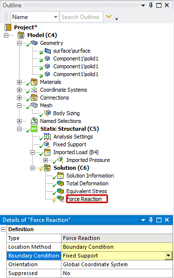
We also want to add a forces resultant in order to validate the coupling between Rocky and Mechanical.
From the Outline panel, right-click Solution, point to Insert, point to Probe, and then click Force Reaction.
From the Details of "Force Reaction" panel, define both Location Method and Boundary Condition.
Now we can solve the FEA portion of the coupled project.
From the Outline panel, right-click Solution, and then click Solve.
The FEA simulation starts processing.
When the simulation concludes, the effects caused by the particles on the surfaces can be easily seen:
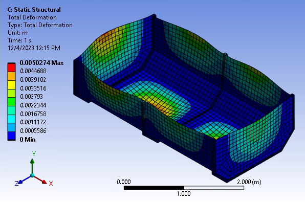
Under Solution, select Total Deformation and then view the results (as shown).
Repeat for Equivalent Stress (as shown).
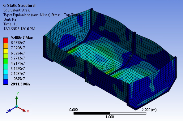
The static structural analysis provides the stress and deformation responses given the particle load for the assessment of the structural integrity of the bin.
The Equivalent (von-Mises) Stress analysis provides information on where the structure can fail due to high stress levels on the surface.
The Total Deformation analysis helps to identify the regions with higher displacements and possible issues with contacting geometries.
We can also evaluate the forces.
Under Solution, select Force Reaction and then view the results for Y Axis.
Reminder: Your results might differ slightly from those shown in this tutorial.

When compared to the Force_Y values we collected in Rocky in Part A (shown above), we can observe a good agreement between the values, which indicates that the loads were correctly interpolated.
Note: Some differences might be observed due to the interpolation methods used.
Close the Static Structural analysis and go back to Workbench.
Now that our initial simulations are complete, let's view what parameters we can vary for our next iterations.
In Ansys Workbench, double-click the Parameter Set block.
From the Parameter Set tab, select the Outline of All Parameters window.
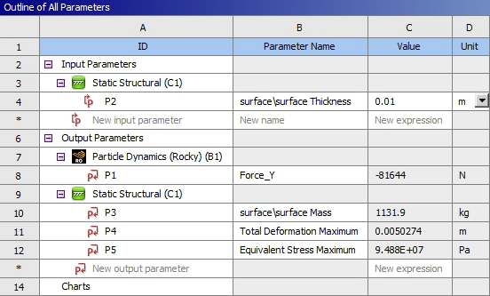
Here, all the parameters created during the analysis are listed, no matter in which application they were created or if they are input or output parameters.
Such input and output parameters can be directly changed to create different scenarios in Workbench.
This provides you valuable information on how to improve your design.
For example, it is possible to parametrize and investige the influence of:
Bin design quantities in Discovery, such as the overall shape of the bin, the number and position of bin supports, and so on.
Particle-related quantities in Rocky, such as material density, tonnage, the particle geometry, the particle size distribution, and so on.
Bin structural quantities in Mechanical, such as the material properties of the bin, the resulting stress and strain, and so on.
Parameter variations can be made in Workbench manually using Design Points (see Tutorial 15 for a walkthrough example of this method) or automatically using Design Exploration.
For this tutorial, we will use the latter method to optimize our bin design.
Our optimization goal is to reduce the mass of the bin as much as safely possible without compromising the structure.
We will accomplish this by setting an objective and then defining constraints on the input and output parameters we exposed in Mechanical.
The optimization problem for this case can be defined as follows:
Single-objective function: Minimize the surface Mass of the bin
Constraint: Equivalent Stress Maximum of the bin should be less than 1e+08 Pa
Free parameter: Bin surface Thickness can range between 0.001 - 0.020 m
Workbench will then use Design Exploration to search for feasible solutions to the problem as defined.
Let's start by defining a new Direct Optimization study.
Switch back to the Project tab.
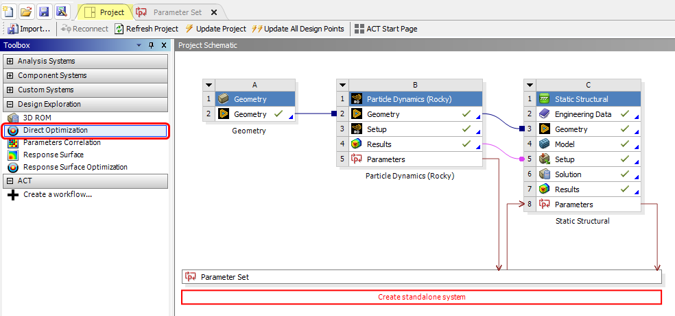
From the Toolbox panel, under Design Exploration, drag Direct Optimization onto the Project Schematic, and drop it under the Parameter Set block.
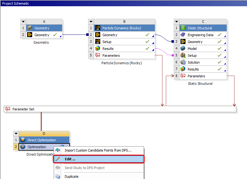
From the new Direct Optimization block, right-click the Optimization component, and then click Edit.
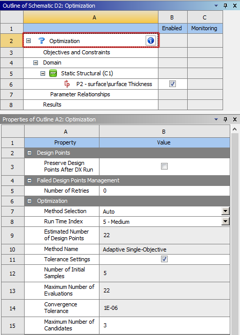
From the Outline of Schematic D2: Optimization window, select the first Optimization item.
From the Properties of Outline A2: Optimization window, review the settings but keep all parameters set as default (as shown).
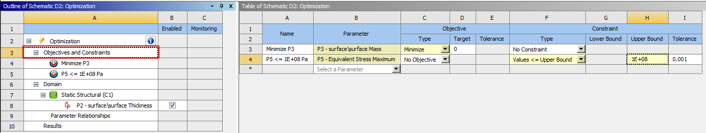
From the Outline of Schematic D2: Optimization window, select the Objectives and Constraints item (as shown).
From the Table of Schematic D2: Optimization window, from the 3rd row, define the Parameter and Objective Type (as shown).
From the 4th row, define the Parameter, Constraint Type, and Constraint Upper Bound (as shown).
From the Outline of Schematic D2: Optimization window, under Domain | Static Structural (C1), select the P2 - surface\surface Thickness item.
From the Table of Schematic D2: Optimization window, from the 3rd row, define the Lower Bound and Upper Bound values (as shown).

Click the Update button to run the optimization cases.

Note: Because many new coupled cases are being calculated, this optimization step can take some time to complete.
Many coupled DEM-FEA cases are run using different parameters that are varied within the constraints set (around 20 scenarios).
As the various cases complete, you can see the parameter values that were used and what results were achieved using those values.
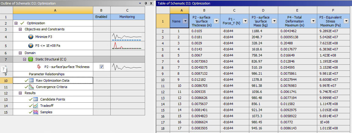
From the Outline of Schematic D2: Optimization window, select Raw Optimization Data (as shown).
From the Table of Schematic D2: Optimization window, notice that each case that completes and its parameter values are listed in a separate row.
When all the cases are complete, we can view the final results.
From the Outline of Schematic D2: Optimization window, under Results, select Samples (as shown).
View information on the Table of Schematic D2: Optimization window (as shown).
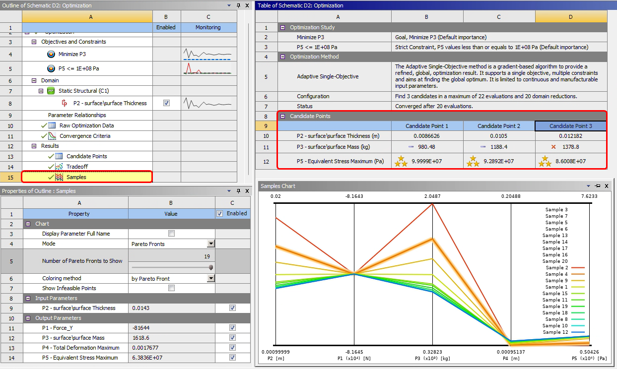
Based upon these results, we can make the following conclusions:
The three cases with values most closely aligning with the objective and constraints are considered Candidates.
Candidate Point 1 (dark blue plot line) shows that by reducing the surface Thickness to 0.0086 m, the surface Mass can be reduced to 980.48 kg while still keeping within the Equivalent Stress Maximum threshold we defined.
As Candidate Point 1 represents the highest stress value allowed for this design optimization, another Candidate that allows for slightly more mass but results in lower stress values might be chosen instead.
This completes Part B of this tutorial.
Through Ansys Workbench, Ansys Static Structural - Mechanical was used to set up and run a FEA simulation using the particle forces calculated previously by Rocky.
During this tutorial, it was possible to:
Make the Rocky DEM results available to Mechanical
Set up and process the FEA simulation in Mechanical
Use key input and output parameters in Workbench to set up and run new optimization cases in Design Exploration
What's Next? If you completed this part successfully, then you are ready to move on to the next tutorial.