


(Part A) Set up and process a simulation using 1-Way coupling between Rocky (DEM) and LBM.
(Part B) Learn how to visualize air flow using vectors and velocity contours, and isolate high-velocity air flow cells using User Processes.
The purpose of this tutorial is to set up and process a simulation using the 1-Way coupling abilities within Rocky, between DEM and the Lattice-Boltzmann Method (LBM).
This method is a useful tool for comparing how equipment design affects the flow of dust and air due to particle interactions.
Important: This ADVANCED tutorial contains fewer details, screenshots, and procedures than other Rocky tutorials.
An ADVANCED tutorial is designed for users who are more familiar with the Rocky user interface (UI), and already have a good understanding of the common setup and post-processing tasks.
If you do not already have this level of familiarity, it is recommended that you complete at least Tutorials 01- 05 before beginning this one.

The geometries in this tutorial are composed of:
(1) Feed Conveyor
(2) Surface
The first item will come from a conveyor template within Rocky. The second item's .stl file can be found in the tutorial directory.
To get started with this tutorial, do the following:
Download the
dem_tut11_files.zipfile here .Unzip
dem_tut11_files.zipto your working directory.Open Rocky 2025 R2.
Create a new project.
Save the empty project to a location of your choosing.
Use the information in the tables that follow to start setting up your Rocky project.
Tip: If you run into settings or procedures in these tables that you are not yet familiar with, please refer to the Rocky User Manual and/or other Tutorials (via the Introductory Tutorials and Advanced Tutorials) to find the detailed instructions you need.
| Step | Data Entity | Editors Location | Parameter or Action | Settings |
|---|---|---|---|---|
| A | Study | Study | Study Name | LBM |
| B | Physics | Physics | Momentum | Rolling Resistance Model | Type C: Linear Spring Rolling Limit ⯆ |
| Numerical Softening Factor | 0.1 [ - ] | |||
| C | Geometries | Import Wall | surface.stl with "mm" for Import Unit | |
| D | Geometries | Create Feed Conveyor | ||
| E | Geometries ﹂Feed Conveyor <01> | Feed Conveyor | Orientation | Belt Incline Angle | 20 [dega] |
| Vertical Offset | 0.2 [m] | |||
| Feed Conveyor | Feeder Box | Drop Box Length | 1.8 [m] | ||
| Drop Box Width | 1.8 [m] | |||
| F | Materials ﹂Default Boundary | Material | Density | 1400 [kg/m3] |
| G | Materials ﹂Default Particles | Materials | Use Bulk Density | (Cleared) |
| Density | 2800 [kg/m3] | |||
| H | Materials Interactions | … | Default Particles ⯆ Default Particles ⯆ | Static Friction | 0.4 [ - ] |
| Dynamic Friction | 0.35 [ - ] | |||
| I | Particles | Create Particle | ||
| J | Particles ﹂Particle <01> | Particle | Movement | Rolling Resistance | 0.2 [ - ] |
| K | Inlets and Outlets | Create Particle Inlet | ||
| L | Inlets and Outlets ﹂Particle Inlet<01> | Particle Inlet | Entry Point | Feed Conveyor <01> ⯆ |
| … | Particles | Add row (x1) | |||
| (1) Particle | Mass Flow Rate | Particle <01> @ 2000 [t/h] | |||
Tip: For more information about setting up a Feed Conveyor, refer to Tutorial 06 – High Pressure Grinding Roll (HPGR).
For the CFD Coupling step, we will turn on and then set up the 1-Way LBM air flow model.
This model is useful for simulating how air and dust flow are affected by the flow of particles in the simulation.
Tip: For more information on how Rocky calculates boundary conditions, see the paper by Verberg and Ladd. [1]
The properties that are able to be adjusted when this model is enabled are described below.
Operation Properties
Use Air Flow: Enables/Disables Lattice-Boltzmann Air Flow calculations.
Start When Particles Enter: Enables air flow calculations to start as soon as particles appear in the air flow limit box.
Air Properties
Air Density: The density of the air.
Air Kinematic Viscosity: The kinematic viscosity of the air.
Lattice-Boltzmann Details
Cell Size: The size of the Air Flow cell.
Interaction Scale: Determines the interaction between the Particle and the air.
Start Time: Disabling the Start When Particles Enter option makes the Start Time parameter available. This is the time that Air Flow calculations begin during the simulation.
Speed of Sound: The speed of sound, which is used to calculate Air Flow.
Boundary Conditions: Method applied for the calculations, affecting accuracy and stability.
Coordinate Limits: The domain limits of the Air flow box.
To set up the CFD Coupling, do the following:
From the Data panel, right-click LBM (Study). From Models, navigate to Enable CFD Coupling and select 1-Way LBM (Particle → Fluid).

Note: You can also enable CFD Coupling options from the main Study menu.
From the Data panel, find the CFD Coupling entity that appears, select the 1-Way LBM entry, and then from the Data Editors panel, modify the parameters as described on the next slide.
From the main 1-Way LBM tab, define the Cell Size, Interaction Scale, and Coordinate Limits (as shown).

Note: The Coordinate Limits can be different than the DEM domain limits.
The Interaction Scale was increased from the original default value (0.25) to reduce the simulation time for the purposes of the tutorial.
Tip: In most cases, it is recommended that you use the default Interaction Scale number.
For the Domain Settings step, we will define a custom boundary box that exceeds the limits of our geometries.
Tip: To learn more about setting boundary limits for your domain, refer to Tutorial 03 – Vibrating Screen.
Use the information in the table that follows to finish setting up your project.
Step Data Entity Editors Location Parameter or Action Settings A Domain Settings Domain Settings Use Boundary Limits (Cleared) Max Values 20, 10, 10 [m] B Solver Solver | General Simulation Target CPU ⯆
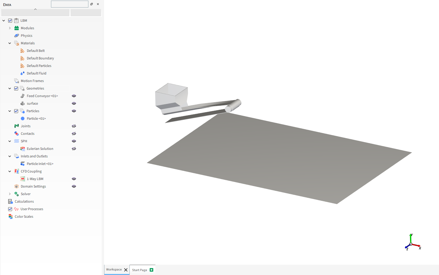
With a 3D View window opened, your Data panel and Workspace should look similar to the below image.
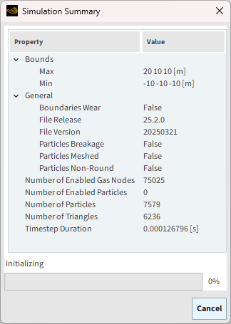
From the Solver entity, click Start.
The Simulation Summary screen appears (as shown), then processing begins.

Tip: You can use the Auto Refresh checkbox to view in a 3D View window the results during processing.
This completes Part A of this tutorial, during which Rocky was used to set up and process a simulation using the Lattice-Boltzmann Method (LBM) Air Flow model.
What's Next?
Now that you have set up and processed this simulation, you are ready to move on to Part B and post-process this project.
The purpose of this tutorial is to use the results from the 1-Way LBM (Lattice-Boltzmann Method) simulation we set up and processed in Part A to analyze how particle flow influences air flow in and around the equipment.
Reminder: The LBM method is a useful tool for comparing how equipment design affects the flow of dust and air due to particle interactions.
You will learn how to:
Visualize air flow using vectors
Analyze velocity contours
Isolate high-velocity air flow cells
And you will use these features:
Air flow vector visualization
Plane User Process
Property User Process
Important: This ADVANCED tutorial contains fewer details, screenshots, and procedures than other Rocky tutorials.
An ADVANCED tutorial is designed for users who are more familiar with the Rocky user interface (UI), and already have a good understanding of the common setup and post-processing tasks.
If you do not already have this level of familiarity, it is recommended that you complete at least Tutorials 01- 05 before beginning this one.
If you completed Part A of this tutorial, ensure that Rocky project is open. (Part B will continue from where Part A left off.)
If you did not complete Part A, do all of the following:
Download the
dem_tut11_files.zipfile here .Unzip
dem_tut11_files.zipto your working directory.Open Rocky 2025 R2. (Look for Rocky 2025 R2 in the Program Menu or use the desktop shortcut.)
Important: To make use of the Rocky project file provided, you must have Rocky 2025 R2 or later. If you have an earlier version of Rocky, please upgrade Rocky to the latest version, or complete Part A from scratch.
From the Rocky program, click the Open Project button, find the dem_tut11_files folder, then from the tutorial_11_A_pre-processing folder, open the tutorial_11_A_pre-processing.rocky file.
Process the simulation. (From the Data panel, select Solver and then from the Data Editors panel, click the Start button.)
One way to visualize the effects of particles upon the air flow is to use vectors.
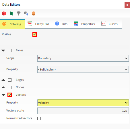
From the Data panel, under CFD Coupling, select the 1-Way LBM entity.
From the Data Editors panel, select the Coloring tab and then ensure both the Visible and Vectors checkboxes are enabled.
Under Vectors, select Velocity from the Property list, and ensure the Vectors scale is 0.25 (as shown).

You can also analyze the velocity contours of a cross section of the air flow by creating a cut plane.
From the Data panel, right-click 1-Way LBM, point to Processes, and then click Plane.
From the Data Editors panel, on the Plane tab, define Orientation (Angle and Vector, as shown).


After the cut plane is defined, switch to the Properties tab and then drag and drop Velocity: Absolute onto the 3D View window.
Tip: To see only the velocity contour, use the Data panel eye icons hide Particles and the 1-Way LBM vectors from the view.

To identify which regions around the equipment are affected most by air flow, you can use a Filter User Process to isolate air flow cells containing velocity values above a certain threshold.
Set up this analysis by using the information in the table below.
Step Data Entity Editors Location Parameter or Action Settings A CFD Coupling ﹂1-Way LBM
Create a Filter User Process B User Processes | Filter <01>
Property Property Velocity: Absolute Type Range Minimum Value 0.5 [m/s] Maximum Value 10 [m/s] After the cells have been isolated, from the Properties tab, drag and drop Velocity: Absolute onto the 3D View.
Tip: To see only the selected cells and Particles, you may need to use the eye icons on the Data panel to hide the Plane <01> User Process and show the Particles entity.

This completes Part B of this tutorial, in which Rocky was used to post-process a 1-Way LBM (Lattice-Boltzmann Method) simulation by analyzing how particle flow influences air flow in and around equipment.
During this tutorial, it was possible to:
Visualize air flow using vectors
Analyze velocity contours using a cut Plane User Process
Isolate high-velocity air flow cells using a Filter User Process
What's Next?
If you have completed this tutorial successfully, then you are ready to move on to next tutorial.