


You can create additional variables based on existing data. Typical mathematical operations, as well as many special built-in functions, enable you to produce simple or complex equations for new variables. Some built-in functions enable you to use values based on the geometric characteristics of server parts. In general, created variables are available for any process, just like given variables. If you have transient data, a time change will recompute the created variable values.
Often an analysis program produces a set of basic results from which other results can be derived. For example, if a computational fluid dynamics analysis gives you density, momentum and total energy, you can derive pressure, velocity, temperature, mach number, etc. EnSight provides many of these common functions for you, or you can enter the equation(s) and build your own.
As another example, suppose you would like to normalize a given scalar or vector variable according to its maximum value, or according to the value at a particular node. Variable creation enables you to easily accomplish such a task. The more familiar you become with this feature, the more uses you will discover.
EnSight allows variables to be defined at vertices (nodes) or element centers or a single value per case (Case constant) or a single value for each part (Part constant). If a new variable is created from a combination of nodal and element based variables, such a new variable will always be element based. Variable names are limited to 49 characters in length.
Note: Part constants, that are in model files and exist with the same value in all parent parts of a created part - are inherited by created parts. If the value differs, they will become undefined in the created part. However, computed constants per part are not automatically inherited by created parts, and become undefined in the created parts. If a value is desired in the created part(s) for the computed constant per part, one should include the created part as one of the parent parts for the computed constant per part.
Note: Measured Variables are not supported by this functionality.
You cannot select both measured and other parts in order to calculate variables. Model part variable calculations must be handled separately from measured parts.
Note: Recalculating an existing computed variable by changing the input variables to a different kind of variable now has a different behavior from versions 23.1 and before. For example:
Scalar to vector.
Nodal to elemental.
Selecting a different input option that changes the result to a different output. (for example, modifying
EleMetricfrom input option0, which generates a scalar, to input option28, which generates a vector).
EnSight now deletes the existing variable and recalculates it as if it is a new variable using the new input parameters and/or input variables. This is a nuanced change to behavior that is not problematic if there are no dependencies on this variable.
However, if there are dependent part(s), for instance calculating an isosurface with this variable or dependent variable (s), (for example, you have calculated dependent variable(s) using this variable), EnSight will then pop up a dialog asking you permission to delete the dependent part(s) and/or variable(s) prior to proceeding with the deletion and recalculation of the new variable. Click to delete the dependent part(s) and/or variables and the variable and recalculate it. You will then need to recreate the dependent part(s) and/or variable(s) again yourself. Click if you do not want this to happen. You can then calculate a brand-new variable of a different name.
The problem with version 23.1 and earlier is that EnSight did not carefully handle the recalculation of a variable nor protect the situation in which the recalculated variable had dependent part(s) and/or dependent computed variable(s). This resulted in unpredictable behavior (ignoring the calculator evaluate, or executing incorrectly), then generating spurious command language that was risky and unprotected at best, or crashed at worst. Command files run in later versions of EnSight behave as if you clicked . Therefore, it is possible, that running 23.1 and earlier command language on later versions of EnSight, may result in unexpected behavior. For example, past behavior that skipped a recalculation of a variable may now recalculate it. Past behavior that skipped the recalculation of a variable and its dependencies may now delete the dependent part(s) and/or variable(s) as well as the variable and recalculate just the variable, leaving the session bereft of dependent part(s)/variable(s) that need to be manually recreated. You may need to rewrite the older command language or redo the calculations and save the resulting new command language.
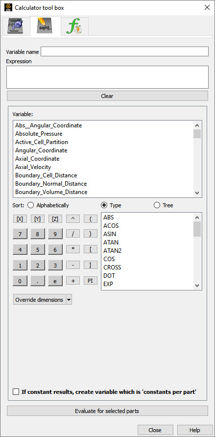
Building Expressions
The Feature Panel (Variables) dialog Variable Creation turn-down section provides function selection lists, calculator buttons, and feedback guidance to aid you in building the working expression (or equation) for a new variable. You can use three types of values in an expression: constants, scalars, and vectors.
Case Constants
| A Case Constant Is a Single Value for That Case | For Example |
|---|---|
| number | 3.56 |
| constant variable from the Active Variables list | Analysis_Time |
| scalar variable at a particular node/element (component and node/element number in brackets) | temperature[25] |
| vector variable component at a particular node /element (component and node/element number in brackets) | velocity[Z][25] |
| coordinate component at a particular node/element (component and node/element number in brackets) | coordinate[X][25] |
| any of the previous three at a particular time step (time step in
braces right after the variable name) Note: This only works for model variables, not created ones. |
temperature{15}[25] velocity{15}[Z][25] coordinate{15}[X][25] |
| Math function | COS(1.5708) |
| General function that produces a constant | AREA(plist) |
Scalars
| A Scalar in a Variable Expression Can Be A | For Example |
|---|---|
| Scalar variable from the Active Variables list | pressure |
| Vector variable component (component in brackets) | velocity[Z] |
| coordinate component (component in brackets) | coordinate[Y] |
| any of the previous three at a particular time step (time step in
braces right after the variable name) Note: This only works for model variables, not created ones. |
pressure{29} velocity{29}[Z] coordinate{29}[Y] |
| General function that produces a scalar | Divergence(plist,velocity) |
Vectors
| A Part Constant Is a Single Value for Each Part | For Example |
|---|---|
| vector variable from the Active Variables list | velocity |
| coordinate name from the Active Variables list | coordinate |
| any of the previous two at a particular time step (time step in
braces right after the variable name) Note: This only works for model variables, not created ones. |
velocity{9} coordinate{9} |
| General function that produces a vector | Vorticity(plist,velocity) |
Part Constants
| A Part Constant Is a Single Value for Each Part | For Example |
|---|---|
| GUI part number part constant | PartNumber() |
| mass flow per part | Flow() |
| mass flow per part at timestep 3 | mass_flow{3} |
The following are some example variable expressions, and how they
can be built. These examples assume Analysis_Time,
pressure, density, and
velocity are all given variables.
| Working Expression | Discussion and How To Build It |
|---|---|
|
-13.5/3.5 |
A true constant since it does not change over time. To build it, type on the keyboard
or click the Variable Creation dialog
calculator buttons |
|
Analysis_Time/60.0 |
A simple example of modifying a given
constant variable. If |
|
velocity*density |
This expression is a vector * scalar, which is momentum, which is a vector. To build it, select velocity from the Active Variables list, type or click *, then select density from the Active Variable list. Note: This means that all vector operations are performed component-wise on each of the components.
|
|
SQRT(pressure[73] * 2.5)+ velocity[X][73] |
This says, take the pressure at node (or
element if pressure is an element center based variable) number
73, multiply it by 2.5, take the square root of the product, and
then add to that the x-component of velocity at node (or
element) number 73. To build it, select SQRT from the
Math function list, select pressure from
the Active Variables list, type |
|
velocity^2 |
You have to be careful here . A vector * vector in EnSight is performed component-wise (x-component * x-component, y-component*y-component, and z-component*z-component). The magnitude of this expression is SQRT(x-component^4 + y-component^4 + z-component^4) which is NOT the square of the magnitude. If you are looking for a scalar result, use SQRT(DOT(velocity,velocity)), or RMS(velocity) or SQRT(velocity[x]*velocity[x] + velocity[y]*velocity[y]+velocity[z]*velocity[z]) |
|
pressure{19} |
This is a scalar, the value of pressure
at time step 19. It does not change with time. To build it,
select pressure from the Active Variables
list, then type Note: Variable must be a model variable, not a computed variable. Do not use a reference to two different timesteps in one calculation as this will slow EnSight down exponentially as it switches back and forth between the timesteps, element by element.
|
|
MAX(plist,pressure) |
MAX is one of the built-in General functions. This expression calculates the maximum pressure value for all the nodes of the selected parts. To build it, type or click (, select MAX from the General function list and follow the interactive instructions that appear in the Feedback area of this dialog (in this case, to select the parts, click OK, and select pressure from the Active Variable list). |
|
pressure^(1.0/3.0) |
The cube root of pressure |
|
/pressure_max)^2 |
This scalar is essentially the normalized
pressure, squared. To build it, first build the preceding
MAX(plist,pressure)
expression and name it |
Notice in the last example how a complex equation can be broken down into several smaller expressions. This is necessary as EnSight can compute only one variable at a time. Calculator limitations include the following:
The variable name cannot be used in the expression.
The following is invalid:
temperature = temperature + 100
Instead use new variable:
temperature2 = temperature + 100
The result of a function cannot be used in an expression.
The following is invalid:
norm_press_sqr = (pressure / MAX(plist,pressure))^2
Instead use two steps:
p_max = MAX(plist,pressure)
then:
norm_press_sqr = (pressure / p_max)^2
Neither created parts, changing geometry model parts, computed variables, nor coordinates can be used with a time calculation (using {}). If one of these is selected when you use {}, the calculation will fails with an error message.
If you need to reference a variable at two different times in an equation, do this using temporary variables. This is because the calculator will compute these values element by element and will find itself switching back and forth in time and will slow down exponentially.
var{5} - var{0}will run exponentially slow as ensight switches back and forth between timestep 0 and timestep 5, element by element.Instead, use the following intermittent variables:
temp5 = var{5}temp0 = var{0}temp5 - temp0Because calculations occur only on server based parts, client based parts are ignored when included in the part list of the pre-defined functions, and variable values may be undefined.
Clicking the Calculator icon opens the Feature Panel (Calculator) dialog.
Predefined Functions
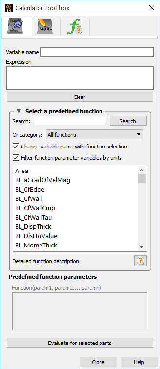
Build Your Own Functions
The EnSight calculator functions are listed below. All of the calculator functions are threaded except as follows. ElemToNode * , Lambda2, MassedParticle, MatSpecies, MatToScalar, NormC, OffsetVar, Q_criteria, Radiograph_grid, Radiograph_mesh, SOSConstant, StatRegVal1, StatRegVal2, TempMean, TempMinmaxField. All of the Math functions are threaded. For more details on this topic see Threading.
Note: The ElemToNode function can enable threading (see
the function description below for details).
Variable units are discussed in a previous section (see Variable Units). The
EnSight calculator is integrated into the unit system in two ways. First,
variables generated via pre-defined functions and the general expression system
will have appropriate unit dimensions generated for them. When the resulting
variable units are unknown, or the expression is invalid, the resulting variable
will appear unitless (unit dimensions = "/"). For example, the simple expression
Coordinates[X] + TEMPERATURE, where
TEMPERATURE has the unit dimensions
K is, from a units perspective, invalid (one cannot
add variables of type L and K)
so the resulting variable would be unitless. Whereas the expression
Coordinates[X] / TEMPERATURE is valid and will have
the unit dimensions L/K.
Some predefined functions may require careful treatment. For
example, consider variables: MakeScalNode(plist,1.0) which
will generate a unitless variable (1.0 has no units). If one needed a nodal
variable of specific dimensionality, one can first create a constant variable
with the appropriate units and pass it to the predefined function. The variable
resulting from MakeScalNode(plist, v) will have the same
units as the constant variable v.
An additional feature of the calculator general expression system can
help simplify the creation of a constant (or any variable) with specific unit
dimensions. If any general expression ends with the @ symbol, the characters
after the @ will be used to explicitly set the variable unit dimensions,
overriding the dimensions computed by default. For example, the expression:
1.0@L/T will create a new constant with the value
of 1 and the units of velocity. The calculator graphical user interface has a
simple interface for previewing and setting these values.
Choose Override dimensions.
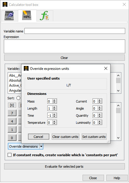
The Override dimensions menu can be used
to bring up the dialog shown here as well as simply set the dimensions to common
values which will be shown as follows: Velocity (@L/T)
or Density (@M/LLL).
The other calculator units feature relates to the predefined function editor. In this editor, where variable selection occurs, the variables are (by default) filtered to only those variables with unit dimensions that are appropriate for the argument. For example, only the variables with M/LT dimensions are displayed for viscosity.
Note: Viscosity is filtered using variable dimensions.
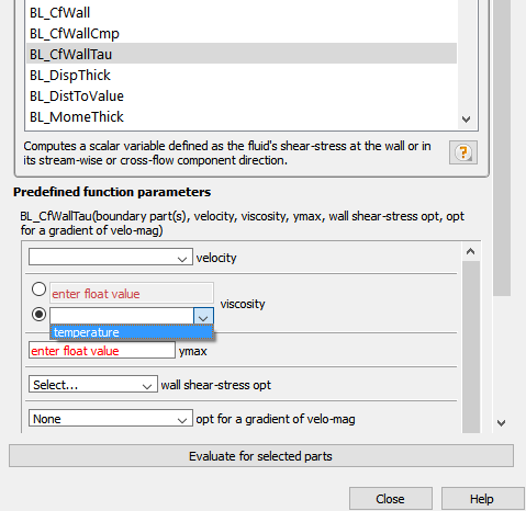
Note: The expected units for other arguments (for example, velocity) are also displayed in the current unit system in the dialog. This filtering can be disabled with the Filter variables by units check box as needed.
Unit conversions are performed as part of server I/O operations. All data in memory (client and server) will be in the session unit system. This ensures that datasets from different sources that might have overlapping variable names will always be consistently displayed in the client. One implication of this is that files saved from EnSight (context files, geometric entities export, etc) will all be written in the session unit system. For example, the geometric entities case gold file export writes out the unit system from the current session (including the metadata files), not in the original source dataset unit system.
The following topics are included in this section:
- 8.5.2.1. Area
- 8.5.2.2. Boundary Layer: A Gradient Of Velocity Magnitude
- 8.5.2.3. Boundary Layer: Edge Skin-Friction Coefficient
- 8.5.2.4. Boundary Layer: Wall Skin-Friction Coefficient
- 8.5.2.5. Boundary Layer: Wall Skin-Friction Coefficient Components
- 8.5.2.6. Boundary Layer: Wall Fluid Shear-Stress
- 8.5.2.7. Boundary Layer: Displacement Thickness
- 8.5.2.8. Boundary Layer: Distance to Value from Wall
- 8.5.2.9. Boundary Layer: Momentum Thickness
- 8.5.2.10. Boundary Layer: Scalar
- 8.5.2.11. Boundary Layer: Recovery Thickness
- 8.5.2.12. Boundary Layer: Shape Parameter
- 8.5.2.13. Boundary Layer: Thickness
- 8.5.2.14. Boundary Layer: Velocity at Edge
- 8.5.2.15. Boundary Layer: off Wall
- 8.5.2.16. Boundary Layer: Distance off Wall
- 8.5.2.17. Case Map
- 8.5.2.18. Case Map Diff
- 8.5.2.19. Case Map Image
- 8.5.2.20. Coefficient
- 8.5.2.21. Complex
- 8.5.2.22. Complex Argument
- 8.5.2.23. Complex Conjugate
- 8.5.2.24. Complex Imaginary
- 8.5.2.25. Complex Modulus
- 8.5.2.26. Complex Real
- 8.5.2.27. Complex Transient Response
- 8.5.2.28. Constant Per Part
- 8.5.2.29. Curl
- 8.5.2.30. Porosity Characterization Functions (Defects)
- 8.5.2.31. Density
- 8.5.2.32. Log of Normalized Density
- 8.5.2.33. Normalized Density
- 8.5.2.34. Normalized Stagnation Density
- 8.5.2.35. Stagnation Density
- 8.5.2.36. Distance Between Nodes
- 8.5.2.37. Distance to Parts: Node to Nodes
- 8.5.2.38. Distance to Parts: Node to Elements
- 8.5.2.39. Divergence
- 8.5.2.40. Element Metric
- 8.5.2.41. Element Size
- 8.5.2.42. Element to Node
- 8.5.2.43. Element to Node Weighted
- 8.5.2.44. Energy: Total Energy
- 8.5.2.45. Kinetic Energy
- 8.5.2.46. Enthalpy
- 8.5.2.47. Normalized Enthalpy
- 8.5.2.48. Stagnation Enthalpy
- 8.5.2.49. Normalized Stagnation Enthalpy
- 8.5.2.50. Entropy
- 8.5.2.51. Flow
- 8.5.2.52. Flow Rate
- 8.5.2.53. Fluid Shear
- 8.5.2.54. Fluid Shear Stress Max
- 8.5.2.55. Force
- 8.5.2.56. Force 1D
- 8.5.2.57. Gradient
- 8.5.2.58. Gradient Tensor
- 8.5.2.59. Helicity Density
- 8.5.2.60. Relative Helicity
- 8.5.2.61. Filtered Relative Helicity
- 8.5.2.62. Iblanking Values
- 8.5.2.63. IJK Values
- 8.5.2.64. Integrals: Line Integral
- 8.5.2.65. Integrals: Surface Integral
- 8.5.2.66. Integrals: Volume Integral
- 8.5.2.67. Length
- 8.5.2.68. Line Integral
- 8.5.2.69. Line Vectors
- 8.5.2.70. Lambda2
- 8.5.2.71. Mach Number
- 8.5.2.72. Make Scalar at Elements
- 8.5.2.73. Make Scalar from Element Ids
- 8.5.2.74. Make Scalar at Nodes
- 8.5.2.75. Make Scalar from Node IDs
- 8.5.2.76. Make Vector
- 8.5.2.77. Massed Particle Scalar
- 8.5.2.78. Mass-Flux Average
- 8.5.2.79. MatSpecies
- 8.5.2.80. MatToScalar
- 8.5.2.81. Max
- 8.5.2.82. Min
- 8.5.2.83. Moment
- 8.5.2.84. MomentVector
- 8.5.2.85. Momentum
- 8.5.2.86. Node Count
- 8.5.2.87. Node to Element
- 8.5.2.88. Normal
- 8.5.2.89. Normal Constraints
- 8.5.2.90. Normalize Vector
- 8.5.2.91. Offset Field
- 8.5.2.92. Offset Variable
- 8.5.2.93. Part Number
- 8.5.2.94. Pressure
- 8.5.2.95. Pressure Coefficient
- 8.5.2.96. Dynamic Pressure
- 8.5.2.97. Normalized Pressure
- 8.5.2.98. Log of Normalized Pressure
- 8.5.2.99. Stagnation Pressure
- 8.5.2.100. Normalized Stagnation Pressure
- 8.5.2.101. Stagnation Pressure Coefficient
- 8.5.2.102. Pitot Pressure
- 8.5.2.103. Pitot Pressure Ratio
- 8.5.2.104. Total Pressure
- 8.5.2.105. Q_criteria
- 8.5.2.106. Radiograph_grid
- 8.5.2.107. Radiograph_mesh
- 8.5.2.108. Rectangular To Cylindrical Vector
- 8.5.2.109. Server Number
- 8.5.2.110. Shock Plot3d
- 8.5.2.111. Mesh Smoothing
- 8.5.2.112. SOS Constant
- 8.5.2.113. Spatial Mean
- 8.5.2.114. Spatial Mean Weighted
- 8.5.2.115. Speed
- 8.5.2.116. Sonic Speed
- 8.5.2.117. Statistics Moments
- 8.5.2.118. Statistics Regression
- 8.5.2.119. Statistics Regression Info
- 8.5.2.120. Statistics Regression Info
- 8.5.2.121. sumPerPart
- 8.5.2.122. sumPerPartArg
- 8.5.2.123. Swirl
- 8.5.2.124. Temperature
- 8.5.2.125. Normalized Temperature
- 8.5.2.126. Log of Normalized Temperature
- 8.5.2.127. Stagnation Temperature
- 8.5.2.128. Normalized Stagnation Temperature
- 8.5.2.129. Temporal Mean
- 8.5.2.130. Temporal Minmax Field
- 8.5.2.131. Tensor Component
- 8.5.2.132. Tensor Determinant
- 8.5.2.133. Tensor Eigenvalue
- 8.5.2.134. Tensor Eigenvector
- 8.5.2.135. Tensor Make
- 8.5.2.136. Tensor Make Asymmetric
- 8.5.2.137. Tensor Tresca
- 8.5.2.138. Tensor Von Mises
- 8.5.2.139. udmf_sum
- 8.5.2.140. Vector 1D Projection
- 8.5.2.141. Vector Cyl Projection
- 8.5.2.142. Vector Rect Projection
- 8.5.2.143. Velocity
- 8.5.2.144. Volume
- 8.5.2.145. Volume Integral
- 8.5.2.146. Vorticity
- 8.5.2.147. Vorticity Gamma
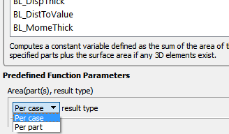
Area (any part(s) [,
Compute_Per_part])
Computes a constant or constant per part variable whose value is the area of the selected parts. If a part is composed of 3D elements, the area is of the border representation of the part. The area of 1D elements is zero.
BL_aGradOfVelMag (boundary part(s), velocity)
Computes a vector variable which is the gradient of the magnitude of the specified velocity variable on the selected boundary part(s) defined as:

where:

| on boundary part |

| velocity vector |

| magnitude of velocity vector = 
|
| x, y, z | coordinate directions |
| i, j, k | unit vectors in coordinate directions |
Note: For each boundary part, this function finds its corresponding field part (pfield), computes the gradient of the velocity magnitude on the field part (Grad(pfield,velocity), and then maps these computed values onto the boundary part.
Node or element IDs are used if they exist. Otherwise the coordinate values between the field part and boundary part are mapped and resolved via a floating-point hashing scheme.
This velocity-magnitude gradient variable can be used as an argument for the following boundary-layer functions that require this variable.
The Boundary Layer Calculator functions
(BL_*) are not supported for Server of Server (SOS)
decomposition Boundary Layer Variables.
Function Arguments
| Boundary part | 2D part |
| Velocity | Vector variable |
BL_CfEdge (boundary part(s), velocity, density,
viscosity, ymax, flow comp(0,1,or2), grad)
Computes a scalar variable which is the edge skin-friction
coefficient  (that is, using the density
  and velocity
  values at the edge of the boundary layer - not the free-stream
density
values at the edge of the boundary layer - not the free-stream
density  and velocity
  values) defined as:
Component: 0 = Total tangential-flow (parallel) to wall:

Component: 1 = Stream-wise (flow) component tangent (parallel) to wall:

Component: 2 = Cross-flow component tangent (parallel) to wall:

where:
|
| fluid shear stress magnitude at the boundary 
|
|
| stream-wise component of 
|
|
| cross-flow component of 
|
|
| dynamic viscosity of the fluid at the wall |
|
| magnitude of the velocity-magnitude gradient in the normal direction at the wall |
|
| stream-wise component of the velocity-magnitude gradient in the normal direction at the wall |
|
| cross-flow component of the velocity-magnitude gradient in the normal direction at the wall |
|
| density at the edge of the boundary layer |
|
| velocity at the edge of the boundary layer |


Function Arguments
|
boundary part |
2D part |
|
velocity |
vector variable |
|
density |
scalar variable (compressible flow), constant number (incompressible flow) |
|
viscosity |
scalar variable, constant variable, or constant number |
|
ymax |
constant number > 0 = Baldwin-Lomax-Spalart algorithm 0 = convergence algorithm (See Algorithm Note under Boundary Layer Thickness) |
|
flow comp |
constant number 0 = tangent flow parallel to surface 1 = stream-wise component tangent (parallel) to wall 2 = cross-flow component tangent (parallel) to wall |
|
grad |
-1 = flags the computing of the velocity-magnitude gradient via 3-point interpolation. vector variable = Grad(velocity magnitude), see Boundary Layer: A Gradient Of Velocity Magnitude Note: Graphical User Interface selection for this option will list
|
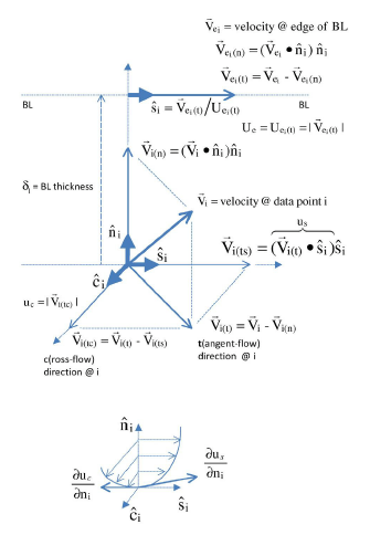
Provides a measure of the skin-friction coefficient in the tangent (parallel to surface) direction, and in its tangent's respective stream-wise and cross-flow directions, respective to the decomposed velocity parallel to the surface at the edge of the boundary layer.
This is a non-dimensionalized measure of the fluid shear
stress at the surface based on the local density and velocity at the edge of the
boundary layer. The following figure illustrates the derivations of the computed
'edge' related velocity values  ,
,  ,
,  &
&  .
.
Note: The Boundary Layer Calculator
functions (BL_*) are not supported for Server of Server
(SOS) decomposition Boundary Layer Variables.
BL_CfWall (boundary part(s), velocity, viscosity, free
density, free velocity, grad)
Computes a scalar variable which is the skin-friction
coefficient  , defined as:

where:
|
|
fluid shear stress at the wall |
|
|
dynamic viscosity of the fluid at the wall May be spatially and/or temporarily varying quantity (usually a constant). |
|
|
distance profiled normal to the wall |
|
|
freestream density |
|
|
freestream velocity magnitude |
|
|
tangent (parallel to surface) component of the velocity-magnitude gradient in the normal direction under the "where:" list. |


This is a non-dimensionalized measure of the fluid shear stress at
the surface. An important aspect of the Skin Friction Coefficient is that
 indicates boundary layer separation.
Function Arguments
|
boundary part |
2D part |
|
velocity |
vector variable |
|
viscosity |
scalar variable, constant variable, or constant number |
|
free density |
constant number |
|
free velocity |
constant number |
|
grad |
-1 = flags the computing of the velocity-magnitude gradient via 3-point interpolation. vector variable = Grad(velocity magnitude), see Boundary Layer: A Gradient Of Velocity Magnitude Note: Graphical User Interface selection for this option will list
|
Important: The Boundary Layer Calculator functions
(BL_*) are not supported for Server of Server (SOS)
decomposition Boundary Layer Variables.
BL_CfWallCmp (boundary part(s), velocity, viscosity,
free-stream density, free-stream velocity-mag., ymax, flow comp(1or2),
grad)
Computes a scalar variable which is a component of the
skin-friction coefficient Cf tangent (or parallel) to the wall, either in the stream-wise
 or in the cross-flow Cfc(·)
 direction defined as:
Component 1 = Stream-wise (flow) component tangent (parallel) to wall:

Component 2 = Cross-flow component tangent (parallel) to wall:

where:

|
stream-wise component of |

|
cross-flow component of |
|
| fluid shear stress magnitude at the wall 
|
|
| dynamic viscosity of the fluid at the wall |
|
| stream-wise component of the velocity-magnitude gradient in the normal direction at the wall |
|
| cross-flow component of the velocity-magnitude gradient in the normal direction at the wall |
|
| density at the edge of the boundary layer |
|
| velocity at the edge of the boundary layer |


Function Arguments
|
boundary part |
2D part |
|
velocity |
vector variable |
|
viscosity |
scalar variable, constant variable, or constant number |
|
density |
scalar variable (compressible flow), constant number (incompressible flow) |
|
velocity mag |
constant variable, or constant number |
|
ymax |
constant number > 0 = Baldwin-Lomax-Spalart algorithm 0 = convergence algorithm (See Algorithm Note under Boundary Layer Thickness) |
|
flow comp |
constant number 1 = stream-wise component tangent (parallel) to wall 2 = cross-flow component tangent (parallel) to wall |
|
grad |
-1 = flags the computing of the velocity-magnitude gradient via 3-point interpolation. vector variable = Grad(velocity magnitude), see Boundary Layer: A Gradient Of Velocity Magnitude Note: Graphical User Interface selection for this option will list
|
Important: The Boundary Layer Calculator functions (BL_*) are not supported for Server of Server (SOS) decomposition Boundary Layer Variables.
BL_CfWallTau (boundary part(s), velocity, viscosity,
ymax, flow comp(0,1,or 2), grad).
Computes a scalar variable which is the fluid's
shear-stress at the wall  or in its stream-wise
  , or cross-flow
  component direction defined as:
Component 0 = Total fluid shear-stress magnitude at the wall:

Component 1 = Stream-wise component of the fluid shear-stress at the wall:

Component 2 = Cross-flow component of the fluid shear-stress at the wall:

where:

|
dynamic viscosity of the fluid at the wall |
|
| magnitude of the velocity-magnitude gradient in the normal direction at the wall |
|
| stream-wise component of the velocity-magnitude gradient in the normal direction at the wall |
|
| cross-flow component of the velocity-magnitude gradient in the normal direction at the wall |


Function Arguments
|
boundary part |
2D part |
|
velocity |
vector variable |
|
viscosity |
scalar variable, constant variable, or constant number |
|
ymax |
constant number > 0 = Baldwin-Lomax-Spalart algorithm 0 = convergence algorithm (See Algorithm Note under Boundary Layer Thickness) |
|
flow comp |
constant number 0 = RMS of the stream-wise and cross-flow components 1 = stream-wise component at the wall 2 = cross-flow component at the wall |
|
grad |
-1 = flags the computing of the velocity-magnitude gradient via 3-point interpolation. vector variable = Grad(velocity magnitude), see Boundary Layer: A Gradient Of Velocity Magnitude Note: Graphical User Interface selection for this option will list
|
Important: The Boundary Layer Calculator functions
(BL_*) are not supported for Server of Server (SOS)
decomposition Boundary Layer Variables.
BL_DispThick (boundary part(s), velocity, density,
ymax, flow comp(0,1,or 2), grad).
Computes a scalar variable which is the boundary-layer
displacement thickness  ,
,  , or
, or  defined as:
Component: 0 = Total tangential-flow parallel to the wall

Component: 1 = Stream-wise flow component tangent (parallel) to the wall

Component: 2 = Cross-flow component tangent (parallel) to the wall

|
|
distance profiled normal to the wall |
|
|
boundary-layer thickness (distance to edge of boundary layer) |
|
|
density at given profile location |
|
|
density at the edge of the boundary layer |
|
|
magnitude of the velocity component parallel to the wall at a given profile location in the boundary layer |
|
|
stream-wise component of the velocity magnitude parallel to the wall at a given profile location in the boundary layer |
|
|
cross-flow component of the velocity magnitude parallel to the wall at a given profile location in the boundary layer |
|
|
u at the edge of the boundary layer |
|
|
distance from wall to freestream |
|
comp |
flow direction option |
|
grad |
flag for gradient of velocity magnitude |


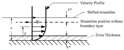
Provides a measure for the effect of the boundary layer on the outside flow. The boundary layer causes a displacement of the streamlines around the body.
Function Arguments
|
boundary part |
2D part |
|
velocity |
vector variable |
|
density |
scalar variable (compressible flow), constant number (incompressible flow) |
|
|
constant number > 0 = Baldwin-Lomax-Spalart algorithm 0 = convergence algorithm (See Algorithm Note under Boundary Layer Thickness) |
|
flow comp |
constant number: 0 = total tangential flow direction parallel to wall 1 = stream-wise flow component direction parallel to wall 2 = cross-flow component direction parallel to wall |
|
grad |
-1 = flags the computing of the velocity-magnitude gradient via 4-point interpolation. vector variable = Grad(velocity magnitude), see Boundary Layer: A Gradient Of Velocity Magnitude Note: Graphical User Interface selection for this option will list
|

Important: The Boundary Layer Calculator functions
(BL_*) are not supported for Server of Server (SOS)
decomposition Boundary Layer Variables.
BL_DistToValue (boundary part(s), scalar, scalar
value).
Computes a scalar variable which is the distance
 from the wall to the specified value defined as:

|
|
distance profile d normal to boundary surface |
|
|
scalar field (variable) |
|
|
scalar field values |
|
|
scalar value at which to assign d |


Function Arguments
|
boundary part |
0D, 1D, or 2D part |
|
scalar |
scalar variable |
|
scalar value |
constant number or constant variable |
Important: The Boundary Layer Calculator functions
(BL_*) are not supported for Server of Server (SOS)
decomposition Boundary Layer Variables.
BL_MomeThick (boundary part(s), velocity, density,
ymax, flow compi(0,1,or2), flow compj(0,1,or2), grad).
Computes a scalar variable which is the boundary-layer
momentum thickness  ,
,  ,
,  ,
,  , or
, or  defined as:
Components: (0,0) = Total tangential-flow parallel to the wall

Components: (1,1) = stream-wise, stream-wise component

Components: (1,2) = Stream-wise, cross-flow component

Components: (2,1) = cross-flow, stream-wise component

Components: (2,2) = cross-flow, cross-flow component

where:
|
|
distance profiled normal to the wall |
|
|
boundary-layer thickness (or distance to edge of boundary layer) |
|
|
density at given profile location |
|
|
density at the edge of the boundary layer |
|
|
magnitude of the velocity component parallel to the wall at a given profile location in the boundary layer |
|
|
stream-wise component of the velocity magnitude parallel to the wall at a given profile location in the boundary layer |
|
|
cross-flow component of the velocity magnitude parallel to the wall at a given profile location in the boundary layer |
|
|
u at the edge of the boundary layer |
|
|
distance from wall to freestream |
|
|
first flow direction option |
|
|
second flow direction option |
|
grad |
flag for gradient of velocity magnitude |


Relates to the momentum loss in the boundary layer.
Function Arguments
|
boundary part |
2D part |
|
velocity |
vector variable |
|
density |
scalar variable (compressible flow), constant number (incompressible flow) |
|
ymax |
constant number > 0 = Baldwin-Lomax-Spalart algorithm 0 = convergence algorithm (See Algorithm Note under Boundary Layer Thickness) |
|
compi |
0 = total tangential flow direction parallel to wall 1 = stream-wise flow component direction parallel to wall 2 = cross-flow component direction parallel to wall |
|
compj |
constant number 0 = total tangential flow direction parallel to wall 1 = stream-wise flow component direction parallel to wall 2 = cross-flow component direction parallel to wall |
|
grad |
-1 = flags the computing of the velocity-magnitude gradient via 4-point interpolation. vector variable = Grad(velocity magnitude), see BL_aGradfVelMag Note: Graphical User Interface selection for this option will list
|
Important: The Boundary Layer Calculator functions
(BL_*) are not supported for Server of Server (SOS)
decomposition Boundary Layer Variables.
BL_Scalar (boundary part(s), velocity, scalar, ymax,
grad).
Computes a scalar variable which is the scalar value of the corresponding scalar field at the edge of the boundary layer. The function extracts the scalar value while computing the boundary-layer thickness (see Boundary Layer: Thickness).
Function Arguments
|
boundary part |
2D part |
|
velocity |
vector variable |
|
scalar |
scalar variable |
|
ymax |
constant number > 0 = Baldwin-Lomax-Spalart algorithm 0 = convergence algorithm (See Algorithm Note under Boundary Layer Thickness) |
|
grad |
-1 = flags the computing of the velocity-magnitude gradient via 4-point interpolation. vector variable = Grad(velocity magnitude) Note: Graphical User Interface selection for this option will list
|
Important: The Boundary Layer Calculator functions
(BL_*) are not supported for Server of Server (SOS)
decomposition Boundary Layer Variables.
BL_RecoveryThick (boundary part(s), velocity, total
pressure, ymax, grad).
Computes a scalar variable which is the boundary-layer
recovery thickness  defined as:

|
|
distance profiled normal to the wall |
|
|
boundary-layer thickness (distance to edge of boundary layer) |
|
|
total pressure at given profile location |
|
|
pt at the edge of the boundary layer |
|
ymax |
distance from wall to freestream |
|
grad |
flag for gradient of velocity magnitude option |


This quantity does not appear in any physical conservation equations, but is sometimes used in the evaluation of inlet flows.
Function Arguments
|
boundary part |
2D part |
|
velocity |
vector variable |
|
total pressure |
scalar variable |
|
ymax |
constant number > 0 = Baldwin-Lomax-Spalart algorithm 0 = convergence algorithm (See Algorithm Note under Boundary Layer Thickness) |
|
grad |
-1 = flags the computing of the velocity-magnitude gradient via 4-point interpolation. vector variable = Grad(velocity magnitude), see BL_aGradfVelMag Note: Graphical User Interface selection for this option will list
|
Important: The Boundary Layer Calculator functions
(BL_*) are not supported for Server of Server (SOS)
decomposition Boundary Layer Variables.
BL_Shape is not explicitly listed in the
general function list, but can be computed as a scalar variable via the
calculator by dividing a displacement thickness by a momentum thickness:

|
|
boundary-layer displacement thickness |
|
|
boundary-layer momentum thickness |


Used to characterize boundary-layer flows, especially to indicate potential for separation.
This parameter increases as a separation point is approached, and varies rapidly near a separation point.
Note: Separation has not been observed for H < 1.8, and definitely has been observed for H = 2.6; therefore, separation is considered in some analytical methods to occur in turbulent boundary layers for H = 2.0.
In a Blasius Laminar layer (for example, a flat plate boundary layer growth with zero pressure gradient), H = 2.605. Turbulent boundary layer, H ~= 1.4 to 1.5, with extreme variations ~= 1.2 to 2.5.
BL_Thick (boundary part(s), velocity, ymax, grad).
Computes a scalar variable which is the boundary-layer thickness
 defined as:

The distance normal from the surface to where:
 ,
,
|
|
magnitude of the velocity component parallel to the wall at a given location in the boundary layer |
|
|
magnitude of the velocity just outside the boundary layer |


.
Function Arguments
|
boundary part |
2D part |
|
velocity |
vector variable |
|
ymax |
constant number > 0 = Baldwin-Lomax-Spalart algorithm 0 = convergence algorithm (See Algorithm Note below) |
|
grad |
-1 = flags the computing of the velocity-magnitude gradient via 3-point interpolation. vector variable = Grad(velocity magnitude), see BL_aGradfVelMag Note: Graphical User Interface selection for this option will list
|
Important: The Boundary Layer Calculator functions
(BL_*) are not supported for Server of Server (SOS)
decomposition Boundary Layer Variables.
Note: Algorithm Note: The ymax argument allows the edge of the boundary layer to be approximated by two different algorithms, for example the Baldwin-Lomax-Spalart and convergence algorithms. Both schemes profile velocity data normal to the boundary surface, or wall. Specifying ymax > 0 leverages results from both the Baldwin-Lomax and vorticity functions over the entire profile to produce a fading function that approximates the edge of the boundary layer. Whereas, specifying ymax = 0 uses velocity and velocity gradient differences to converge to the edge of the boundary layer.
See the following references for more detailed explanations.
P.M. Gerhart, R.J. Gross, & J.I. Hochstein, Fundamentals
of Fluid Mechanics, 2nd Ed.,(Addison-Wesley: New York,
1992)
P. Spalart, A Reasonable Method to Compute Boundary-Layer
Parameters from Navier-Stokes Results, (Unpublished: Boeing,
1992)
H. Schlichting & K. Gersten, Boundary Layer Theory, 8th
Ed., (Springer-Verlag: Berlin, 2003)
BL_VelocityAtEdge (boundary part(s), velocity,
ymax,comp(0,1,2),grad).
Extracts a vector variable which is a velocity vector
 ,
,  , or
, or  defined as:

|
 = velocity vector at the edge of the boundary
layer = velocity vector at the edge of the boundary
layer 
|

|
 = the decomposed velocity vector normal to the
wall at the edge of the boundary layer = the decomposed velocity vector normal to the
wall at the edge of the boundary layer 
|

|
 = the decomposed velocity vector parallel to
the wall at the edge of the boundary layer = the decomposed velocity vector parallel to
the wall at the edge of the boundary layer 
|
Computes a scalar variable which is the boundary-layer thickness
 defined as:

|
 = the decomposed velocity vector normal to the
wall at the edge of the boundary layer = the decomposed velocity vector normal to the
wall at the edge of the boundary layer
|

|
 = the decomposed velocity vector parallel to
the wall at the edge of the boundary layer = the decomposed velocity vector parallel to
the wall at the edge of the boundary layer
|
Computes a scalar variable which is the boundary-layer
thickness defined as:
|
boundary part |
2D part |
|
velocity |
vector variable |
|
density |
scalar variable (compressible flow), constant number (incompressible flow) |
|
ymax |
constant number > 0 = Baldwin-Lomax-Spalart algorithm 0 = convergence algorithm (See Algorithm Note under Boundary Layer Thickness) |
|
comp |
constant number 0 = velocity vector at edge of boundary layer 1 = decomposed velocity vector parallel to wall tangent to surface 2 = decomposed velocity vector normal to wall |
|
grad |
-1 = flags the computing of the velocity-magnitude gradient via 4-point interpolation. vector variable = Grad(velocity magnitude), see BL_aGradfVelMag Note: Graphical User Interface selection for this option will list
|
Important: The Boundary Layer Calculator functions
(BL_*) are not supported for Server of Server (SOS)
decomposition Boundary Layer Variables.
BL_Y1Plus (boundary part(s), density, viscosity, grad
option, vector variable).
 Computes a scalar variable which is the coefficient off the
wall to the first field cell centroid, defined as:
Computes a scalar variable which is the coefficient off the
wall to the first field cell centroid, defined as:

where:
|
|
distance profiled normal to the wall |
|
|
|
|
|
dynamic viscosity of fluid at wall May be spatially and/or temporally varying quantity (usually a constant) |
|
|
density at the wall |
|
|
distance from first field element centroid to outer face, profiled normal to wall |
|
|
fluid velocity vector |


Normally  is used to estimate or confirm the required 1st grid spacing
for proper capturing of viscous-layer properties. The values are dependent on
various factors including, what variables at the wall are sought, the turbulent
models used, and whether the law of the wall is used or not. Consult a
boundary-layer text for correct interpolation of the values for your
application.
is used to estimate or confirm the required 1st grid spacing
for proper capturing of viscous-layer properties. The values are dependent on
various factors including, what variables at the wall are sought, the turbulent
models used, and whether the law of the wall is used or not. Consult a
boundary-layer text for correct interpolation of the values for your
application.
Function Arguments
|
boundary part |
2D (wall or surface) part |
|
density |
scalar variable |
|
viscosity |
scalar variable, constant variable, or constant number |
|
gradient option |
1. Use field velocity (will be used to calculate wall gradient) 2. Use gradient at boundary part (wall or surface) 3. Use gradient in corresponding field part |
|
vector variable |
Will be one of three depending on gradient option 1. Use field velocity = velocity vector 2. Use gradient at boundary = Gradient variable on 2d boundary (wall or surface) part 3. Use gradient in field = Gradient variable defined in 3D field part; or could be gradient calculated using Grad(velocity magnitude), see BL_aGradfVelMag |
Important: The Boundary Layer Calculator functions
(BL_*) are not supported for Server of Server (SOS)
decomposition Boundary Layer Variables.
BL_Y1PlusDist (boundary part(s), velocity).
 Computes a scalar variable which is the off-the-wall distance,
 , which is the distance off the wall to the first field cell
centroid. The velocity variable is only used to determine whether the variable
is nodal or elemental to maintain consistency with the
, which is the distance off the wall to the first field cell
centroid. The velocity variable is only used to determine whether the variable
is nodal or elemental to maintain consistency with the  calculation above.
Function Arguments
|
boundary part |
2D part |
|
velocity |
vector variable |
Important: The Boundary Layer Calculator functions
(BL_*) are not supported for Server of Server (SOS)
decomposition Boundary Layer Variables.
CaseMap (2D or 3D part(s), case to map from,
scalar/vector/tensor, parts to map from, search option flag)
For all locations on the selected part(s) this function finds the specified variable value (scalar, vector, or tensor) from the case to map from using a variety of user-specified search options. If the variable in the case to map from is located at the nodes, then the casemapped variable will be defined on the nodes of the selected part(s), and if the variable is located at the elements, then the casemapped variable will be defined at the elements of the selected part(s).
The idea is to map onto the selected part(s), a variable from another case, usually for comparison purposes. It does this by taking the location of the nodes or centroid of the elements and looking at the other case to see if the variable in question is defined at that location in the field. If so, the value is mapped to the parts nodes or element value. The algorithm can be fairly expensive, so there are options to inform the search that finds a matching variable location.
There are several options available in this function that can greatly impact the performance as follows.
|
case to map from |
constant number |
|
scalar/vector/tensor |
scalar, vector, or tensor variable |
|
search option |
If mapping search is successful, always assigns the exact value found. If search mapping is not successful, because there is not an exact match of node or element location, then the following occurs: If search option is set to search only (0), an undefined value will be assigned. If search option is set to 'nearest value' (1), the defined variable value at the closest node or element will be assigned (so no undefined values). This option will take time to search the 'from case' according to the 'parts to map from" selection outlined below. |
|
parts to map from |
The values for a location must be found by searching the geometry in the 'case to map from'. By setting this option you can hint to EnSight where in the geometry it should search, which can vastly improve performance. Global search - This is the legacy scheme which will perform a methodical, but uninformed search of the 3D, then 2D, then 1D, then even 0D (point) elements to find the first defined variable value. This works well for mapping onto a 3D or 2D that is completely enclosed in a 3D from volume. It works poorly if the 2D is not fully enclosed (such as on the edge of a 3D part) or if you want to map a 2D onto a 2D part and other 3D parts exist. Dimensionality match - Only parts of the same dimension in the from and to are searched. For example, only 3D from parts will be used to map onto a 3D selected part. This is the option that you should use most often. Part number match - The order of the parts is used, that is if you are computing the case map on the third part then the third part is used in the 'case to map from'. This is best used if you have exactly the same dataset in terms of the part list ordering, but perhaps calculated differently so only the variable values differ. Parts selected for case to map from - Select parts in the Case From as well as the Case To. Only selected parts will be used in the two cases. |
Note: This function uses EnSight's search capability to do the mapping. It is critical that the nodes of the parts being mapped onto, lie within the geometry of all of the parts of the case being mapped from. Mapping from a 2D surface to a 2D surface will only work reliably if the surfaces are the same (or extremely close, and the flag=1 option is chosen). Mapping nodal variables is faster than mapping elemental variables. This function is threaded so an Enterprise (formerly gold or hpc) license key may improve performance. Select only the parts that you require, and use search option 0 if at all possible. For more details, see Compare Cases, and for detailed pointers see Case Mapping Tips in that same How To write up.
Example 8.1: Case Map Scenario
I have a 2D part in case 1 that I want to case map a variable from a similar 2D part in case 2. First, select the 2D part in from case 1 in the Part List. Then set case to map from to 2 and set the variable you want to map in the calculator pulldown. Then use the search option 'nearest value' (=1) to mitigate tolerance issues between the 2D part surfaces. Now the fourth option depends on the data in the two cases. You should choose Global search if you only have one 2D part in case 2 (because there is only one part to search in the case). If, however, there are multiple parts (with some 3D parts) in case 2, do not use the Global search because it will waste time searching first in the 3D parts before it searches the 2D parts. Choose Part number match if the 2D parts are in the same location in the Part List for both cases (for example, both are second in their respective cases). Or, choose Dimensionality match to limit the search to only the 2D parts in case 2. Or you could choose the option Parts selected for case to map from and you would then select the 2D part in the case to map from AND the 2D part in both case 1 and case 2, thereby limiting the search to only the one 2D part.
Important: Case mapping functions are not supported for Server of Server (SOS) decomposition because SOS was designed to benefit from independent Servers computations in parallel. The inter-dependent computational mapping of the field results from the fluid part onto the boundary part violates this assumption. You cannot be sure that you will have all of the fluid information on one server for the mapping, so this is disabled.
CaseMapDiff (2D or 3D part(s), case to map from,
scalar/vector/tensor, 0/1 0=search only 1=if search fails find closest)
This function is equivalent to Variable -
CaseMap[Variable]. See CaseMap function
for details on how that function works.
See Compare Cases.
CaseMapImage (2D or 3D part(s), part to map from,
scalar, viewport number, Undefined value limit)
This Function does a projection of a 2D part variable from a different case onto a 3D geometry taking into account the view orientation from the specified viewport number, similar to a texture mapping. The function in effect maps 2D results to a 3d geometry taking into account view orientation and surface visibility.
Function Arguments
|
part to map from |
Part number of the 2D part. This 2D part is usually data from an infrared camera. |
|
scalar |
scalar variable |
|
viewport number |
The viewport number showing part(s) the variable is being computed on, from the same camera view as part to map from |
|
Undefined value limit |
Values on the 2D part that are under this value are considered Undefined |
Note: If the variable in the part to map from is located at the nodes, then
the casemapped variable will be at the nodes. If the
variable is located at the elements the casemapped
variable will be at the elements. This function takes only a scalar
variable.
Coeff (any 1D or 2D part(s), scalar, component)
Computes a constant or constant per part variable whose
value is a coefficient  ,
,  , or
, or  such that
  ,
,  ,
,
where:
|
| any scalar variable |
|
| 1D or 2D domain |
|
| x component of normal |
|
| y component of normal |
|
| z component of normal |


Function Arguments
| variable | scalar or vector |
| component | if variable is a vector: [X], [Y], or [Z] |
Specify [X], [Y], or [Z] to get the corresponding coefficient.
Note: Normal for a 1D part will be parallel to the plane of the plane tool.
Cmplx (any part(s), scalar/vector(real portion),
scalar/vector(complex portion), [optional frequency(Degrees)])
Creates a complex scalar or vector from two scalar or vector variables. The frequency is optional and is used only for reference.
Z = A + Bi
Function Arguments
|
real portion |
scalar or vector variable |
|
complex portion |
scalar or vector variable (but must be same as real portion) |
|
[frequency] |
constant number (optional) |
CmplxArg (any part(s), complex scalar or vector)
Computes the Argument of a complex scalar or vector. The resulting scalar is given in degrees and will be in the range -180 and 180 degrees.

CmplxConj (any part(s), complex scalar or vector)
Computes the Conjugate of a complex scalar of vector. Returns a complex scalar or vector where:


CmplxImag (any part(s), complex scalar or
vector)
Extracts imaginary portion of a complex scalar or vector into a real scalar or vector.

CmplxModu (any part(s), complex scalar or vector)
Returns a real scalar/vector which is the modulus of the given scalar/vector

CmplxReal (any part(s), complex scalar or vector)
Extracts the real portion of a complex scalar or vector into a real scalar or vector.

CmplxTransResp (any part(s), complex scalar or vector,
constant PHI(0.0-360.0 Degrees))
Returns a real scalar or vector which is the real transient response:

which is a function of the transient phase angle
 defined by:

where:
|
t | the harmonic response time parameter |
|
f | frequency of the complex variable
|
and the complex field  , defined as:

where:
|
Vc | the complex variable field |
|
Re(Vc) | the Real portion of Vc |
|
Im(Vc) | the imaginary portion of Vc |
|
i | Sqrt(-1) |
Note: The transient complex function, was a composition of Vc and Euler's relation, namely
Vt = Vt(x,y,z,t) = Re(Vt) + i Im(Vt) = Vc * e^(i phi)
where:
e^(i phi) = Cos(phi) + i Sin(phi)
The real portion Re(Vt), is as designated above:
This function is only good for harmonic variations, producing fields with a defined frequency.
Function Arguments
|
phi angle |
constant number between 0 and 360 degrees. |
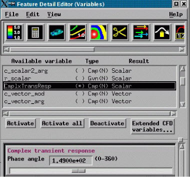
Note: A special area becomes available in the Feature Panel (Variables) and Feature Panel (Calculator) when you highlight a variable of this type - allowing you to modify the phase angle (phi) easily with a slider.
ConstantPerPart (any part(s),
constant)
This function is assigns a value to the selected part(s). The value can either be a floating point value entered into the field, or it can be a case constant. This value does not change over time. At a later point, any other part(s) can be selected and this can be recalculated and these other part(s) will be assigned the new value and the exisiting part(s) that were previously selected will retain their previously assigned value. Each successive time that this is recalculated for an existing variable, values assigned to the most recently selected parts are updated without removing previously assigned values.
Curl (any part(s), vector)
Computes a vector variable which is the curl of the input vector

Consider a mesh with a scalar per element variable representing the micro porosity of each cell, where 0 means no porosity (the cell is completely full) and 100 means the cell is fully porous (the cell is empty). Cells with a non zero porosity are considered to have defects. Defects that span multiple cells may indicate an unacceptable defect.
Six Defect functions are provided to help calculate factors of interest in characterizing
these defects that occur over multiple cells. To use the Defect_*
functions, you would create an isovolume of your porosity variable
between desired ranges (perhaps 5 to 100) and select this isovolume part.
Then use these functions:
Defect_BulkVolume (2D or
3D part(s))
Returns a per element scalar which is the sum of the volume of all the cells comprising the defect, and then each cell with the defect is assigned this value.
See Porosity Characterization Functions (Defects) for further input specifications.
Defect_Count (2D or 3D
part(s), Defect scalar per elem, min value, max
value)[,Compute_Per_part])
Returns a case constant which filters the count of the number of defects that exist between the min value and the max value using a Defect scalar per element variable that has been previously calculated by any of the other five Defect functions.
See Porosity Characterization Functions (Defects) for further input specifications.
Defect_LargestLinearExtent
(2D or 3D part(s))
Returns a per element scalar that is the largest linear extent of all the cells comprising the defect, where each cell of the defect is assigned this value. The largest linear extent is the root-mean-squared distance.
See Porosity Characterization Functions (Defects) for further input specifications.
Defect_NetVolume (2D or 3D
part(s), scalar per elem, scale factor)
Returns a per element scalar that is the sum of the cell volumes multiplied by the scalar per element variable multiplied by the scale factor, of all the cells comprising the defect, where each cell of the defect is assigned this value. The defect scalar per element variable is usually porosity, but the user is free to use any per element scalar variable. The scale factor adjusts the scalar per element variable values, for example if the porosity range is from 0.0 to 100.0 then a scale factor of 0.01 can be used to normalize the porosity values to volume fraction values ranging from 0.0 to 1.0.
See Porosity Characterization Functions (Defects) for further input specifications.
Defect_ShapeFactor (2D or
3D part(s))
Returns a per element scalar that is the Largest Linear Extent divided by the diameter of the sphere with a volume equal to the Bulk Volume of the defect, where each cell of the defect is assigned this value.
See Porosity Characterization Functions (Defects) for further input specifications.
Defect_SurfaceArea (2D or
3D part(s))
Returns a per element scalar that is the surface area of the defect, where each cell of the defect is assigned this value.
See Porosity Characterization Functions (Defects) for further input specifications.
Density (any part(s), pressure, temperature, gas
constant)
Computes a scalar variable which is the density
 , defined as:

where:

| pressure |

| temperature |

| gas constant |
Function Arguments
| pressure | scalar variable |
| temperature | scalar variable |
| gas constant | scalar, constant, or constant per part variable, or constant number |
DensityLogNorm (any part(s), density, freestream
density)
Computes a scalar variable which is the natural log of Normalized Density defined as:

where:

| density |

| freestream density |
Function Arguments
|
density |
scalar variable, constant variable, or constant number |
|
freestream density |
constant or constant per part variable or constant number |
DensityNorm (any part(s), density, freestream density)
Computes a scalar variable which is the Normalized
Density  defined as:

where:

| density |

| freestream density |
Function Arguments
|
density |
scalar variable, constant variable, or constant number |
|
freestream density |
constant or constant per part variable or constant number |
DensityNormStag (any part(s), density,
total energy, velocity, ratio of specific heats, freestream density, freestream
speed of sound, freestream velocity magnitude)
Computes a scalar variable which is the Normalized Stagnation Density defined as:

where:

| stagnation density |

| freestream stagnation density |
where:
|
density |
scalar, constant, or constant per part variable, or constant number |
|
total energy |
scalar variable |
|
velocity |
vector variable |
|
ratio of specific heats |
scalar, constant or constant per part variable, or constant number |
|
freestream density |
constant or constant per part variable or constant number |
|
freestream speed of sound |
constant or constant per part variable or constant number |
|
freestream velocity magnitude |
constant or constant per part variable or constant number |
DensityStag (any part(s), density, total energy,
velocity, ratio of specific heats)
Computes a scalar variable which is the Stagnation
Density  defined as:

where:

| density |
|
| ratio of specific heats |
|
| mach number |


Function Arguments
|
density |
scalar, constant, or constant per part variable, or constant number |
|
total energy |
scalar variable |
|
velocity |
vector variable |
|
ratio of specific heats |
scalar, constant, or constant per part variable, or constant number |
Dist2Nodes (any part(s), nodeID1,
nodeID2)
Computes a constant, positive variable that is the distance between
any two nodes. Searches down the part list until it finds
nodeID1, then searches until it finds
nodeID2 and returns Undef
if nodeID1 or nodeID2 cannot be found.
Nodes are designated by their node ID's, so the part must have node IDs.
Note: Most created parts do not have node IDs
The geometry type is important for using this function. There are three geometry types: static, changing coordinate, and changing connectivity. You can find out your geometry type by doing a Query → Dataset and look in the General Geometric section of the pop up window.
If you have a static geometry with visual displacement turned on then
dis2nodes will not use the displacement in its
calculations. You will need to turn on server-side (computational)
displacement (see Server
Side Displacements). If you have changing coordinate geometry, then
dist2node works without adjustment. if you have
changing connectivity then dist2node should not be used
as it may give nonsensical results because connectivity is re-evaluated each
timestep and node IDs may be reassigned.
For transient results, to find the distance between two nodes on different parts, or between two nodes if one or both don't have IDs, or the IDs are not unique for the model (namely, more than one part has the same node ID) use the line tool. See the Advanced Usage section of Use the Line Tool.
Function Arguments
|
nodeID1 |
constant number |
|
nodeID2 |
constant number |
Dist2Part (origin part + field part(s), origin part,
origin part normal)
Computes a scalar variable on the origin part and field parts that is the minimum distance at each node of the origin and field parts to any node in the origin part. This distance is unsigned by default. The origin part is the origin of a Euclidean distance field. So, by definition the scalar variable will always be zero at the origin part because the distance to the origin part will always be zero.
The origin part normal vector must be a per node
variable. If the origin part normal is calculated using the Normal calculator
function, then it is a per element variable and must be moved to the nodes using
the calculator ElemToNode function. If this per node,
origin part normal vector variable defined at the origin part is supplied then
the normal vector is used to return a signed distance function (with positive
being the direction of the normal). The signed distance is determined using the
dot product of the vector from the given field node and its closest node on the
origin with the origin node's normal vector.
Note: The origin part must be included in the field part list (although, as discussed earlier, the scalar variable will be zero for all nodes on the origin part). This algorithm has an execution time on the order of the number of nodes in the field parts times the number of nodes in the origin part. While the implementation is both SOS aware and threaded, the run time is dominated by the number of nodes in the computation.
This function is computed between the nodes of the
origin and field parts. As a result, the accuracy of its approximation to the
distance field is limited to the density of nodes (effectively the size of the
elements) in the origin part. If a more accurate approximation is required, use
the Dist2PartElem() function. It is slower, but is less
dependent on the nodal distribution in the origin part because it uses the nodes
plus the element faces to calculate the minimum distance.
Usage: A typical usage would be to use an arbitrary 2D
part to create a clip in a 3D field. Use the 2D part as your origin part, and
select the origin part as well as your 3D field parts. No need to have normal
vectors. Create your scalar variable, called say
distTo2Dpart, then create an isosurface=0 in your field using
the distTo2Dpart as your variable.
Function Arguments
|
origin part |
part number to compute the distance to |
|
origin part normal |
a constant for unsigned computation or a nodal vector variable defined on the origin part for a signed computation |
Dist2PartElem (origin part + field part(s), origin
part, origin part normal)
Computes a scalar variable that is the minimum distance at each node of the origin part and field parts and the closest point on any element in origin part. This distance is unsigned (if the origin part normal vector is not supplied).
If the origin part normal vector is supplied, then the distance is signed.
Note: The origin part normal vector must be a per node variable. If the
origin part normal is calculated using the Normal calculator function,
then it is a per element variable and must be moved to the nodes using
the calculator ElemToNode function. If this per
node, origin part normal vector variable defined at the origin part is
supplied, the direction of the normal is used to return a signed
distance function with distances in the direction of the normal being
positive.
Once the closest point in the origin part has been found for a node in an field part, the dot product of the origin node normal and a vector between the two nodes is used to select the sign of the result.
Note: The origin part must be included in the field part list (although the output will be zero for all nodes of the origin part because it is the origin of the Euclidean distance). This algorithm has an execution time on the order of the number of nodes in the field parts times the number of elements in the origin part. While the implementation is both SOS aware and threaded, the run time is dominated by the number of nodes in the computation
This function is a more accurate estimation of the distance field
than Dist2Part() because
it allows for distances between nodes and element surfaces on the origin part.
This improved accuracy results in increased computational complexity and as a
result this function can be several times slower than
Dist2Part().
Function Arguments
|
origin part |
part number to compute the distance to |
|
origin part normal |
a constant for unsigned computation or a nodal vector variable defined on the origin part for a signed computation |
Div (2D or 3D part(s), vector)
Computes a scalar variable whose value is the divergence defined as:

where:
|
u,v,w |
velocity components in the X, Y, Z directions |
EleMetric (any part(s), metric_function).
Calculates an element mesh metric, at each element creating a scalar, element-based variable depending upon the selected metric function. The various metrics are valid for specific element types. If the element is not of the type supported by the metric function, the value at the element will be the EnSight undefined value. Metrics exist for the following element types: tri, quad, tet, and hex. A metric can be any one of the following:
|
# |
Name |
Elem types |
Description |
|
0 |
Element type |
All |
EnSight element type number. See the table below this one. |
|
1 |
Condition |
hexa8, tetra4, quad4, tria3 |
Condition number of the weighted Jacobian matrix. |
|
2 |
Scaled Jacobian |
hexa8, tetra4, quad4, tria3 |
Jacobian scaled by the edge length products. |
|
3 |
Shape |
hexa8, tetra4, quad4, tria3 |
Varies by element type. |
|
4 |
Distortion |
hexa8, tetra4, quad4, tria3 |
Distortion is a measure of how well-behaved the mapping from parameter space to world coordinates is. |
|
5 |
Edge ratio |
hexa8, tetra4, quad4, tria3 |
Ratio of longest edge length over shortest edge length. |
|
6 |
Jacobian |
hexa8, tetra4, quad4 |
The minimum determinate of the Jacobian computed at each vertex. |
|
7 |
Radius ratio |
tetra4, quad4, tria3 |
Normalized ratio of the radius of the inscribed sphere to the radius of the circumsphere. |
|
8 |
Minimum angle |
tetra4, quad4, tria3 |
Minimum included angle in degrees. |
|
9 |
Maximum edge ratio |
hexa8, quad4 |
Largest ratio of principle axis lengths. |
|
10 |
Skew |
hexa8, quad4 |
Degree to which a pair of vectors are parallel using the dot product, maximum. |
|
11 |
Taper |
hexa8, quad4 |
Maximum ratio of a cross-derivative to its shortest associated principal axis. |
|
12 |
Stretch |
hexa8, quad4 |
Ratio of minimum edge length to maximum diagonal. |
|
13 |
Oddy |
hexa8, quad4 |
Maximum deviation of the metric tensor from the identity matrix, evaluated at the corners and element center. |
|
14 |
Max aspect Frobenius |
hexa8, quad4 |
Maximum of aspect Frobenius computed for the element decomposed into triangles. |
|
15 |
hexa8, quad4 |
Minimum of aspect Frobenius computed for the element decomposed into triangles. |
|
|
16 |
Shear |
hexa8, quad4 |
Scaled Jacobian with a truncated range. |
|
17 |
Signed volume |
hexa8, tetra4 |
Volume computed, preserving the sign. |
|
18 |
Signed area |
tria3, quad4 |
Area preserving the sign. |
|
19 |
Maximum angle |
tria3, quad4 |
|
|
20 |
Aspect ratio |
tetra4, quad4 |
Maximum edge length over area. |
|
21 |
Aspect Frobenius |
tetra4, tria3 |
Sum of the edge lengths squared divided by the area and normalized. |
|
22 |
Diagonal |
hexa8 |
Ratio of the minimum diagonal length to the maximum diagonal length. |
|
23 |
Dimension |
hexa8 |
|
|
24 |
Aspect beta |
tetra4 |
Radius ratio of a positively-oriented tetrahedron. |
|
25 |
Aspect gamma |
tetra4 |
Root-mean-square edge length to volume. |
|
26 |
Collapse ratio |
tetra4 |
Smallest ratio of the height of a vertex above its opposing triangle to the longest edge of that opposing triangle across all vertices of the tetrahedron. |
|
27 |
Warpage |
quad4 |
Cosine of the minimum dihedral angle formed by planes intersecting in diagonals. |
|
28 |
All |
Returns each element centroid as a vector value at that element |
|
|
29 |
Volume Test |
3D elements |
Returns 0.0 for non-3D elements. Each 3D element is decomposed into Tet04 elements and this option returns a scalar equal to 0.0, 1.0 or 2.0. It returns 0.0 if none of the Tet04 element volumes is negative, 1.0 if all of the Tet04 element volumes are negative, and 2.0 if some of the Tet04 element volumes are negative. |
|
30 |
Signed Volume |
3D elements |
Returns 0.0 for non-3D elements. Returns a scalar which is the sum of the signed volumes of the Tet4 decomposition for 3D elements. |
|
31 |
Part Number |
All |
Returns a scalar at each element which is the EnSight part ID number of that element. |
|
32 |
Face Count |
All |
Returns a scalar which is the number of faces in that element. |

EnSight Element types:
| # | Element Type |
|---|---|
|
0 |
Point |
|
1 |
Point ghost |
|
2 |
2 node bar |
|
3 |
2 node bar ghost |
|
4 |
3 node bar |
|
5 |
3 node bar ghost |
|
6 |
3 node triangle (tria3) |
|
7 |
3 node triangle ghost |
|
10 |
6 node triangle |
|
11 |
6 node triangle ghost |
|
12 |
4 node quadrilateral (quad4) |
|
13 |
4 node quadrilateral ghost |
|
14 |
8 node quadrilateral |
|
15 |
8 node quadrilateral ghost |
|
16 |
4 node tetrahedron (tetra4) |
|
17 |
4 node tetrahedron ghost |
|
20 |
10 node tetrahedron |
|
21 |
10 node tetrahedron ghost |
|
22 |
5 node pyramid |
|
23 |
5 node pyramid ghost |
|
24 |
13 node pyramid |
|
25 |
13 node pyramid ghost |
|
26 |
6 node pentahedron |
|
27 |
6 node pentahedron ghost |
|
28 |
15 node pentahedron |
|
29 |
15 node pentahedron ghost |
|
30 |
8 node hexahedron (hexa8) |
|
31 |
8 node hexahedron ghost |
|
32 |
20 node hexahedron |
|
33 |
20 node hexahedron ghost |
|
34 |
N-sided polygon |
|
35 |
N-sided polygon ghost |
|
38 |
N-faced polyhedron |
|
39 |
N-faced polyhedron ghost |
The implementation is based on the BSD implementation of the Sandia Verdict Library. See the following links:
http://cubit.sandia.gov/public/documents/Verde_UG-2.5B.pdf Verde User's Manual
Verdict Mesh Verification Library
For more detail on individual metrics, see the following reference:
C. J. Stimpson, C. D. Ernst, P. Knupp, P. P. Pebay, & D.
Thompson, The Verdict Library Reference Manual, May 8,
2007.
EleSize (any part(s)).
Calculates the Volume/Area/Length for 3D/2D/1D elements respectively, at each element creating a scalar, element-based variable.
Important: This will use the coordinates of the element to calculate the volume of each element. If you wish to use displacement in the calculation of the volume, then you must turn on computational (server-side) displacement, rather than visual only (client side) displacement so that the displacement values will be applied to the coordinates on the server prior to calculating the element size (see Display Displacements).
If you calculate the element size of a part and then use that part to create a child part, the child part will inherit the values of the elesize calculation which are the size of the parent elements not the size of the child elements. If you want the elesize of the child part, then you must select the child part and recalculate a new elesize variable!
ElemToNode (any part(s), element-based scalar or
vector).
Averages an element based variable to produce a node-based variable.
For each node[i] → 
For each node[i] → 
Results: node[i] → 
where:
| wt | 1 for this algorithm and the weighting scalar in
ElemtoNodeWeighted
|
| j | iterator on all part elements |
| i | iterator on all part nodes Note: nodes[i] must be on elem[j] to contribute |
| | node[i] |
indicates node that is associated with elem[j] |
By default, this uses all parts that share each node of the selected part(s). So, parts that are not selected whose elements are shared by nodes of the selected part(s) will have their element values averaged in with those of the selected parts.
Note: To turn the averaging across parts off and use only the elements of
the each part at each node, open up the command window
(File → Command)
and, in the Command Entry: field,
type test: across averaging off prior to using
this function. The added benefit of turning averaging between parts off,
is that the function becomes threaded.
ElemToNodeWeighted (any part(s), element-based scalar
or vector, element-based weighting scalar).
Same as ElementToNode, except that the value of the variable at the
element is weighted by an element scalar. That is, elem[j]->wt is the value
of the weighting scalar in the ElemToNode algorithm
description above.
One use of this function might be to use the element size as a weighting factor so that larger elements contribute more to the nodal value than smaller ones.
EnergyT (any part(s), density, pressure, velocity,
ratio of specific heats).
Computes a scalar variable of total energy per unit volume.
 | Total Energy |
 | Internal Energy |
 | Stagnation Energy |
 | density |
 | velocity |
Or based on gamma, pressure and velocity:

Function Arguments
KinEn (any part(s), velocity, density)
Computes a scalar variable whose value is the kinetic
energy  defined as:

where:

| density |

| velocity variable |
Function Arguments
|
velocity |
vector variable |
|
density |
scalar, constant, or constant per part variable, or constant number |
Enthalpy (any part(s), density, total energy, velocity,
ratio of specific heats)
Computes a scalar variable which is Enthalpy
 defined as:


| total energy per unit volume |
|
| density |
|
| velocity magnitude |
|
| ratio of specific heats |


Function Arguments
|
density |
scalar, constant, or constant per part variable, or constant number |
|
total energy |
scalar variable |
|
velocity |
vector variable |
|
ratio of specific heats |
scalar, constant, or constant per part variable, or constant number |
EnthalpyNorm (any part(s), density, total energy,
velocity, ratio of specific heats, freestream density, freestream speed of
sound)
Computes a scalar variable which is Normalized Enthalpy
 defined as:


| enthalpy |
|
| freestream enthalpy |

Function Arguments
|
density |
scalar, constant, or constant per part variable, or constant number |
|
total energy |
scalar variable |
|
velocity |
vector variable |
|
ratio of specific heats |
scalar, constant, or constant per part variable, or constant number |
|
freestream density |
constant or constant per part variable or constant number |
|
freestream speed of sound |
constant or constant per part variable or constant number |
EnthalpyStag (any part(s), density, total energy,
velocity, ratio of specific heats)
Computes a scalar variable which is Stagnation
Enthalpy
 defined as:


| enthalpy |

| velocity magnitude |
|
density |
scalar, constant, or constant per part variable, or constant number |
|
total energy |
scalar variable |
|
velocity |
vector variable |
|
ratio of specific heats |
scalar, constant, or constant per part variable, or constant number |
EnthalpyNormStag (any part(s), density, total energy,
velocity, ratio of specific heats, freestream density, freestream speed of
sound, freestream velocity magnitude)
Computes a scalar variable which is Normalized
Stagnation Enthalpy
 defined as:


| stagnation enthalpy |
|
| freestream stagnation enthalpy |

|
density |
scalar, constant, or constant per part variable, or constant number |
|
total energy |
scalar variable |
|
velocity |
vector variable |
|
ratio of specific heats |
scalar, constant, or constant per part variable, or constant number |
|
freestream density |
constant or constant per part variable or constant number |
|
freestream speed of sound |
constant or constant per parts variable or constant number |
|
freestream velocity magnitude |
constant or constant per part variable or constant number |
Entropy (any part(s), density, total energy, velocity,
ratio of specific heats, gas constant, freestream density, freestream speed of
sound)
Computes a scalar variable which is
Entropy
 defined as:

where:
|
| density |
|
| gas constant |
|
| ratio of specific heats |
|
| freestream speed of sound |
|
| freestream density |


where pressure,  is calculated from the total energy,
  , and velocity

with freestream pressure, 
Function Arguments
|
density |
scalar, constant, or constant per part variable, or constant number |
|
total energy |
scalar variable |
|
velocity |
vector variable |
|
ratio of specific heats |
scalar, constant, or constant per part variable, or constant number |
|
gas constant |
scalar, constant, or constant per part variable or constant number |
|
freestream density |
constant or constant per part variable or constant number |
|
freestream speed of sound |
constant or constant per part variable or constant number |
Flow (any 1D or 2D part(s), velocity
[,Compute_Per_part]).
Computes a constant or constant per part variable whose value is the
volume flow rate  defined as:

where:

| Velocity vector |

| Unit vector normal to surface |

| 1D or 2D domain |
Function Arguments
|
velocity |
vector variable |
Note: The normal for each 2D element is calculated using the right hand rule of
the 2D element connectivity and must be consistent over the part or your
results will be incorrect. Normal for a 1D part will be
parallel to the plane of the plane tool. To calculate mass flow rate,
multiply Velocity vector by the Density
scalar and then substitute this vector value in for the velocity
vector in the above equation.
FlowRate (any 1D or 2D part(s), velocity).
Computes a scalar  which is the component of velocity normal to the surface,
defined as:
which is the component of velocity normal to the surface,
defined as:

where:

| Velocity |

| Unit vector normal to surface |

| 1D or 2D |
Function Arguments
|
velocity |
vector variable |
Note: This function is equivalent to calculating the dot product of the
velocity vector at each location and the surface normal (using the
Normal
function).
FluidShear (2D part(s), velocity magnitude gradient,
viscosity)
Computes a scalar variable tau whose value is defined as:

where:

| shear stress |

| dynamic viscosity |

| Velocity gradient in direction of surface normal |
Tip: To compute fluid shear stress:
Use
Gradientfunction on velocity to obtainVelocity Gradvariable in the 3D part(s) of interest.Create a clip part or extract the outer surface of the part using part extract (create a 2D part from the 3D part(s) used above) a surface on which you wish to see the fluid shear stress.
Compute
Fluid Shearvariable (on the 2D surface).
Function Arguments
|
velocity gradient |
vector variable |
|
viscosity |
scalar, constant, or constant per part variable, or constant number |
FluidShearMax (2D or 3D part(s), velocity, density,
turbulent kinetic energy, turbulent dissipation, laminar viscosity)
Computes a scalar variable  defined as:
 where:

| force |
|
| unit area |
|
| turbulent (eddy) viscosity |
|
| laminar viscosity (treated as a constant) |
|
| local strain |


The turbulent viscosity  is defined as:

where:

| density |
|
| turbulent kinetic energy |
|
| turbulent dissipation |


A measure of local strain  (local elongation in 3 directions) is given by

where:

given the Euclidean norm defined by
 ;
;
and the rate of deformation tensor  defined by

with:

|

|

|

|

|

|

|

|

|

|

|

|
given the strain tensor  defined by
Function Arguments
|
velocity |
vector variable |
|
density |
scalar, constant, or constant per part variable, or constant number |
|
turbulent kinetic energy |
scalar variable |
|
turbulent dissipation |
scalar variable |
|
laminar viscosity |
constant or constant per part variable or constant number |
Force (2D part(s), pressure)
Computes a vector variable whose value is the force
 defined as:

where:

| pressure |

| unit area |
Note: The force acts in the surface normal direction.
Function Arguments
|
pressure |
scalar variable |
Force1D (1D planar part(s), pressure, surface
normal)
Computes a vector variable whose value is the force
 defined as:

where:

| pressure |

| unit length normal vector |
Function Arguments
|
pressure |
scalar variable |
|
surface normal |
vector variable |
Grad (2D or 3D part(s), scalar or vector(Magnitude will
be used))
Computes a vector variable whose value is the gradient
 defined as:

where:

| any scalar variable (or the magnitude of the specified vector) |

| coordinate directions |
|
| unit vectors in coordinate directions |

Algorithm
If the variable is at the element, then it is moved to the nodes. Then each element is mapped to a normalized element and the Jacobian is calculated for the transformation from the element to the normalized element; and then, its inverse Jacobian is calculated for this transformation and used to compute the Jacobian for the scalar variable. Therefore, the chain rule is used with the inverse Jacobian of the transformation and the Jacobian of the scalar variable to calculate the gradient for each node of each element. The contributions of the gradient from all the elements are moved to all the nodes using an unweighted average. Finally, if the original variable is per element, the gradient is moved from the nodes to the elements using an unweighted average.
GradTensor (2D or 3D part(s), vector)
Computes a tensor variable whose value is the gradient
 defined as:

where:

| any vector variable |
|
| coordinate directions |
|
| unit vectors in coordinate directions |


HelicityDensity (any part(s), velocity)
Computes a scalar variable  whose value is:

where:

| velocity |
|
| vorticity |

Function Arguments
|
velocity |
vector variable |
HelicityRelative (any part(s), velocity)
Computes a scalar variable  whose value is:

where:
 | the angle between the velocity vector and the vorticity vector |
| V | velocity |
| Ω | vorticity |
Function Arguments
|
velocity |
vector variable |
HelicityRelFilter (any part(s), velocity, freestream
velocity magnitude).
Computes a scalar variable  whose value is:
 , if
, if  or
or  , if
, if 
where:

| relative helicity (as described above) |
|
| helicity density (as described above) |
| filter | 0.1(V∞)2 |

Function Arguments
|
velocity |
vector variable |
|
freestream velocity magnitude |
constant or constant per part variable or constant number |
IblankingValues (Any iblanked structured
part(s))
Computes a scalar variable whose value is the iblanking flag of selected parts. Returns undefined for unstructured part(s).
IJKValues (Any structured part(s))
Computes a vector variable whose value is the I/J/K values of the selected parts. Returns undefined for unstructured part(s).
IntegralLine (1D part(s), scalar or
(vector, component) [,Compute_Per_part])
Computes a constant or constant per part variable whose value is the integral of the input variable over the length of the specified 1D part(s). Nodal variables are first converted to elemental variable using a weighted average of the shape function.
IntegralSurface (2D part(s), scalar or
(vector, component) [,Compute_Per_part])
Computes a constant or constant per part variable whose value is the integral of the input variable over the surface of the specified 2D part(s). Nodal variables are first converted to elemental variable using a weighted average of the shape function.
IntegralVolume (3D part(s), scalar or
(vector, component) [,Compute_Per_part])
Computes a constant or constant per part variable whose value is the integral of the input variable over the volume of the specified 3D part(s). Nodal variables are first converted to elemental variable using a weighted average of the shape function.
Length (any 1D part(s)
[,Compute_Per_part])
Computes a constant or constant per part variable whose value is the length of selected parts. While any part can be specified, it will only return a nonzero length if the part has 1D elements.
LineVectors (any 1D part(s))
Computes a nodal, vector variable which is the

|
| Vector with origin at point i, with i from 1 to n-1. |
|
| Coordinates of Point i of 1D part |
|
| Number of points in the 1D part |


Lambda2 (any part(s), Grad_Vel_x, Grad_Vel_y,
Grad_Vel_z)
Computes a scalar variable which is the
second eigenvalue, or  , of the second invariant (or Q-criterion) of the velocity
gradient tensor. Vortex shells may then be visualized as an iso-surface of
= 0. The following describes the calculation of the inputs to
this function:
, of the second invariant (or Q-criterion) of the velocity
gradient tensor. Vortex shells may then be visualized as an iso-surface of
= 0. The following describes the calculation of the inputs to
this function:
Explicitly calculate the three components of Velocity
Vel_x = Velocity[X] = x-component of the velocity vector
Vel_y = Velocity[Y] = y-component of the velocity vector
Vel_z = Velocity[Z] = z-component of the velocity vector
and then
Grad_Vel_x = Grad(any part(s), Vel_x) = gradient of x component Velocity
Grad_Vel_y = Grad(any part(s), Vel_y) = gradient of y component Velocity
Grad_Vel_z = Grad(any part(s), Vel_z) = gradient of z component Velocity
where:
| Velocity | velocity vector variable |
Note: A common mistake is to try to calculate the Gradient from the component of the velocity without using the intermediate Vel_x, Vel_y, and Vel_z variables. For example this is wrong and will use only the velocity magnitude:
Grad_Vel_x = Grad(any part(s), Velocity[X])
This is a User-Defined Math Function (UDMF) which may be modified and recompiled by the user. For more details, see the Interface Manual, User Defined Math Functions and see User Defined Math Functions, discussed above.
Algorithm
The three gradient vectors of the components of the
velocity vector constitute the velocity gradient tensor. Using the 9 components
of this (anti-symmetric) velocity gradient tensor, Lv, construct both the
symmetric, S, and the anti-symmetric,  , parts of the velocity gradient tensor,

where:

|

|
| Ω |

|
then combine to compute the symmetric tensor

Next compute and sort the eigenvalues of  (using Jacobi eigen analysis), and assign the 2nd eigenvalue,
or , as the scalar value at the node.
(using Jacobi eigen analysis), and assign the 2nd eigenvalue,
or , as the scalar value at the node.

The vortex is to be visualized as an iso-surface with

See also the Q_criteria calculator function.
References
Haller, G., "An objective definition of a vortex," Journal of
Fluid Mechanics, 2005, vol. 525, pp. 1-26.
Jeong, J. and Hussain, F., "On the identification of a
vortex," Journal of Fluid Mechanics, 1995, vol. 285, pp.
69-94.
Mach (any part(s), density, total energy, velocity,
ratio of specific heats)
Computes a scalar variable whose value is the Mach
number  defined as:

where:

| momentum |
|
| density |
|
| speed, computed from velocity input. |
|
| ratio of specific heats (1.4 for air) |
|
| pressure (see Pressure below) |
|
| speed of sound |


See Energy: Total Energy for a description.
Function Arguments
|
density |
scalar, constant, or constant per part variable, or constant number |
|
total energy |
scalar variable |
|
velocity |
vector variable |
|
ratio of specific heats |
scalar, constant, or constant per part variable, or constant number |
MakeScalElem (any part(s), constant number or constant
or constant per part variable)
Assigns the specified constant value to each element, making a scalar variable.
MakeScalElemId (any part(s))
Creates a scalar variable set to the element IDs of the part. If the element ID does not exist or is undefined the scalar value is set to the Undefined value.
MakeScalNode (any part(s), constant number or constant
or constant per part variable)
Assigns the specified constant value to each node, making a scalar variable.
MakeScalNodeId (any part(s))
Creates a scalar variable set to the node IDs of the part. If the node ID does not exist or is undefined the scalar value is set to the Undefined value.
MakeVect (any part(s), scalar or zero, scalar or zero,
scalar or zero)
Computes a vector variable formed from scalar variables. First scalar becomes the X component of the vector, second scalar becomes the Y component, and the third scalar becomes the Z component. A zero can be specified for some of the scalars, creating a 2D or 1D vector field.
Note: A quick way to make a vector, is to select the parts that you wish to use and then select three scalars, scalar_x, scalar_y, and scalar_z in the variable list and then right-click and choose Make Vector in the pull-down and in the side choose whether to use all (or all available, if you have measured) parts or your currently selected parts (if you have parts selected) to calculate the vector. A vector variable will be calculated and named hopefully adequately using the scalar names.
If the order of the variables or the name of the vector cannot be definitively determined, then a GUI will pop up with the proposed components in a pull-down and a proposed name for the created vector variable.
MassedParticle (massed particle trace part(s))
This scalar creates a massed-particle per element scalar variable for each of the parent parts of the massed-particle traces. This per element variable is the mass of the particle times the sum of the number of times each element is exited by a mass-particle trace. See Particle-Mass Scalar on Boundaries.
MassFluxAvg (any 1D or 2D part(s), scalar,
velocity, density [,Compute_Per_part])
Computes a constant or constant per part variable whose
value is the mass flux average  defined as:

where:
|
| any scalar variable, (pressure, mach, a vector component, and so on) |
|
| density (constant or scalar) variable |
|
| velocity (vector) variable |
|
| area of some 2D domain |
|
| unit vector normal to 
|


Function Arguments
|
scalar |
any scalar variable (pressure, mach, a vector component, and so on) |
|
velocity |
a vector variable |
|
density |
scalar, constant, or constant per part variable, or constant number |
Note: The dot product (V*N), is positive when velocity is aligned with the unit normal vector and is negative otherwise (see the FlowRate calculator function). This implies that aligned flow contributes to the weighted average and otherwise subtracts from it. This also presents the possibility that in recirculating flow, the denominator can tend toward zero. Some prefer to use the absolute value of the dot product, which is a multi-step process using the absolute value of the result from the EnSight FlowRate calculator function.
MatSpecies (any model part(s), any material(s), any
specie(s), scalar per element).
Computes a scalar per element variable whose value
 is the sum of all specified material and species combinations
multiplied by the specified element variable on specified 'model' parts with
defined material species.
is the sum of all specified material and species combinations
multiplied by the specified element variable on specified 'model' parts with
defined material species.

where:

| scalar per element variable value or value |

|
|


This function only operates on model part(s) with pre-defined species. The specified material(s) can either be a list of materials or a single material value. The specified species can either be a list, a single specie, or no specie (for example, a null species list which then computes an element value based on only material fraction contributions). The scalar per element value can either be an active variable, or a scalar value (for example, the value 1 would give pure material fraction and/or specie value extraction).
Both material and specie names are selected from the context sensitive Active Variables list which changes to a Materials list and then a Species List for their respective prompts.
For more information on Species see both Material Section and Example Material Dataset (With Species).
MatToScalar (any model part(s), a material)
Computes a scalar per element variable whose value s is the specified material's value m of the element on the specified part(s).
s = m
where:
| s | scalar per element variable value of each element |
| m | the corresponding material fraction value of each element |
This function only operates on model part(s) with pre-defined materials that are given by sparse mixed material definitions. Only one material may be converted into one per element scalar variable at a time. The material cannot be the null material.
For more information on Materials,(see Material Interface Parts), and both MATERIAL Sections under EnSight Gold Case File Format, and Example Material Dataset in Utility Programs.
Max (any part(s), scalar or (vector, component))
Computes a constant or constant per part variable whose value is the maximum value of the scalar (or vector component) in the parts selected. The component is not requested if a scalar is selected.
|
[component] |
if vector variable, magnitude is the default, or specify [x], [y], or [z] |
Min (any part(s), scalar or (vector, component))
Computes a constant or constant per part variable whose value is the minimum value of the scalar (or vector component) in the parts selected.
|
[component] |
if vector variable, magnitude is the default, or specify [x], [y], or [z] |
Moment (any part(s), vector, component)
Computes a constant or constant per part variable (the
moment about the cursor tool location) whose value is the x, y, or
z component of Moment  .
.


where:

| force vector component in direction i of vector

|
|
|
signed moment arm (the perpendicular
distance from the line of action of the vector component
(which is the current cursor tool position)). |
| vector | any vector variable |
| component | [X], [Y], or [Z] |

MomentVector (any part(s), force vector).
Computes a nodal vector variable (the moment is computed
about each point of the selected parts) whose value is the x, y, or
z component of Moment .
where:
|
| force vector component in direction i of vector
|
|
| signed moment arm (the perpendicular distance from the line
of action of the vector component  to the moment axis (model point
position)). to the moment axis (model point
position)). |
Function Arguments
|
force vector |
any vector variable (per node or per element) |
Momentum (any part(s), velocity, density).
Computes a vector variable  , which is:

where:

| density |

| velocity |
Function Arguments
|
velocity |
a vector variable |
|
density |
scalar, constant, constant per part variable, or constant number |
NodeCount (any part(s)
[,Compute_Per_part])
Produces a constant or constant per part variable containing the node count of the part(s) specified.
NodeToElem (any part(s), node-based scalar or
vector)
Averages a node based variable to produce an element based variable.
For each: elem[j]->val += node[i]->val | elem[j]
Results: elem[j]->val /= elem[j]->num_cell_nodes
where:
| j | iterator on all part elements |
| i | iterator on all part nodes elem[j] indicates element that is associated with node[i] |
Note: elem[j] must contain node[i] to contribute
Normal (2D part(s) or 1D planar part(s))
Computes a vector variable which is the normal to the surface at each element for 2D parts, or for 1D planar parts - lies normal to the 1D elements in the plane of the part.
NormC (2D or 3D part(s), pressure,
velocity, viscosity [,Compute_Per_part])
Computes a constant or constant per part variable whose
value is the Normal Constraints  defined as:

where:

| pressure |
|
| velocity |
|
| dynamic viscosity |
|
| direction of normal |
|
| border of a 2D or 3D domain |


Function Arguments
|
pressure |
scalar variable |
|
velocity |
vector variable |
|
viscosity |
scalar, constant, or constant per part variable, or constant number |
NormVect (any part(s),
vector)
Computes a vector variable whose value is a unit vector
 of the given vector
  .
.

 | vector variable field |
 |  |
OffsetField (2D or 3D
part(s))
Computes a scalar field of offset values. The values will be in model distance units perpendicular to the boundary of the part.
Note:
An isosurface created in this field would mimic the part boundary, but at the offset distance into the field.
This calculator function is not supported for Server of Server (SOS) decomposition because SOS was designed to benefit from independent Servers computations in parallel. The inter-dependent computational mapping of the field results from the fluid part onto the boundary part violates this assumption. You cannot be sure that you will have all of the fluid information on one server for the mapping, so this is disabled.
OffsetVar (2D or 3D part(s), scalar or vector, constant
offset value)
Computes a scalar (or vector) variable defined as the offset value into the field of that variable that exists in the normal direction from the boundary of the selected part. This assigns near surface values of a variable to the surface of the selected part(s) from the neighboring 3D field (which is found automatically using the selected part(s) surface(s).
This function gets the value of a variable from surrounding field(s), a fixed distance from the surface of the selected part(s) and assigns it to the surface fo the selected part. For example, you might use this function to get the value of the velocity in the flow field a slight distance above your vehicle surface and assign that value to your vehicle surface.
To use this function, select part(s) in the part list that you want to use, enter a variable and an offset. EnSight will auto detect the 3D field part(s) adjacent to your selected part(s) surface(s) and reach into these fields by your offset in the normal direction to obtain the variable value and then assign it to the surface of your selected part(s).
Note:
Choose a negative offset if your normals do not point into the field.
This calculator function is not supported for Server of Server (SOS) decomposition because SOS was designed to benefit from independent Servers computations in parallel. Recall that EnSight must find the field adjacent to your selected part(s) surfaces. And since some of these fields might be on other servers, it will create dependencies that preclude independent Servers, so this is disabled.
Function Arguments
|
constant offset value |
constant number (constant variable is not valid) |
PartNumber (any part(s)
[,Compute_Per_part])
Computes a constant per part variable which is the GUI part number, if the part is a server-side part. If computed as ‘Compute_Per_case’, the value will be the maximum part number.
Note: Any client-side part (for example, vector arrows, particle traces, profiles, and so on) are assigned the undefined value. Model parts are always server-side parts. For a listing of which created parts are server-side or client-side, see Part Selection and Identification. For a brief discussion of the undefined value, see EnSight Gold Undefined Variable Values Format.
Pres (any part(s),density, total energy, velocity,
ratio of specific heats)
Computes a scalar variable whose value is the pressure
 defined as:


| momentum |
|
| total energy |
|
| density |
|
|
velocity |
|
| ratio of specific heats (1.4 for air) |


Function Arguments
|
density |
scalar, constant, or constant per part variable, or constant number |
|
total energy |
scalar variable |
|
velocity |
vector variable |
|
ratio of specific heats |
scalar, constant, or constant per part variable, or constant number |
PresCoef (any part(s), density, total energy, velocity, ratio
of specific heats, freestream density, freestream speed of sound, freestream
velocity magnitude)
Computes a scalar variable which is Pressure Coefficient
 defined as:


| pressure |
|
| freestream pressure |
|
| freestream density |
|
| freestream velocity magnitude |


Function Arguments
|
density |
scalar, constant, constant per part variable, or constant number |
|
total energy |
scalar variable |
|
velocity |
vector variable |
|
ratio of specific heats |
scalar, constant, or constant per part variable, or constant number |
|
freestream density |
constant or constant per part variable or constant number |
|
freestream speed of sound |
constant or constant per part variable or constant number |
|
freestream velocity magnitude |
constant or constant per part variable or constant number |
PresDynam (any part(s), density, velocity)
Computes a scalar variable which is Dynamic Pressure
 defined as:

|
| density |
|
| velocity magnitude |


See Kinetic Energy.
Function Arguments
|
density |
scalar, constant, or constant per part variable, or constant number |
|
velocity |
vector variable |
PresNorm (any part(s), density, velocity, ratio of specific
heats, freestream density, freestream speed of sound)
Computes a scalar variable which is Normalized Pressure
 defined as:

where:

| freestream pressure = 
|

| ratio of specific heats |

| pressure |
Function Arguments
|
density |
scalar, constant, or constant per part variable, or constant number |
|
total energy |
scalar variable |
|
velocity |
vector variable |
|
ratio of specific heats |
scalar, constant, or constant per part variable, or constant number |
|
freestream density |
constant or constant per part variable or constant number |
|
freestream speed of sound |
constant or constant per part variable or constant number |
PresLogNorm (any part(s), density, total energy, velocity,
ratio of specific heats, freestream density, freestream speed of sound)
Computes a scalar variable which is the natural log of Normalized Pressure defined as:

|
| freestream pressure =
|
|
| ratio of specific heats |
|
| pressure |
Function Arguments
|
density |
scalar, constant, or constant per part variable, or constant number |
|
total energy |
scalar variable |
|
velocity |
vector variable |
|
ratio of specific heats |
scalar, constant, or constant per part variable, or constant number |
|
freestream density |
constant or constant per part variable or constant number |
|
freestream speed of sound |
constant or constant per part variable or constant number |
PresStag (any part(s), density, total energy, velocity, ratio
of specific heats)
Computes a scalar variable which is the Stagnation
Pressure  defined as:

|
| pressure |
|
| ratio of specific heats |
|
| mach number |


Note: In literature, stagnation pressure is used interchangeably with total pressure. The stagnation pressure (or total pressure) use two different equations depending upon the flow regime: compressible or incompressible. EnSight has chosen to define Stagnation Pressure using the compressible flow equation (above), and Total Pressure using the incompressible flow equation (see Total Pressure below).
Function Arguments
|
density |
scalar, constant, or constant per part variable, or constant number |
|
total energy |
scalar variable |
|
velocity |
vector variable |
|
ratio of specific heats |
scalar, constant, or constant per part variable, or constant number |
PresNormStag (any part(s), density, total energy, velocity,
ratio of specific heats, freestream density, freestream speed of sound,
freestream velocity magnitude)
Computes a scalar variable which is Normalized
Stagnation Pressure 
defined as:

where:

| stagnation pressure |

| freestream stagnation pressure |
Function Arguments
|
density |
scalar, constant, or constant per part variable, or constant number |
|
total energy |
scalar variable |
|
velocity |
vector variable |
|
ratio of specific heats |
scalar, constant, or constant per part variable, or constant number |
|
freestream density |
constant or constant per part variable or constant number |
|
freestream speed of sound |
constant or constant per part variable or constant number |
|
freestream velocity magnitude |
constant or constant per part variable or constant number |
PresStagCoef (any part(s), density, total energy, velocity,
ratio of specific heats, freestream density, freestream speed of sound,
freestream velocity magnitude)
Computes a scalar variable which is Stagnation Pressure
Coefficient 
defined as: 
where:

| stagnation pressure |

| freestream pressure = 
|

| ratio of specific heats |

| freestream density |

| velocity magnitude |
Function Arguments
|
density |
scalar, constant, or constant per part variable, or constant number |
|
total energy |
scalar variable |
|
velocity |
vector variable |
|
ratio of specific heats |
scalar, constant, or constant per part variable, or constant number |
|
freestream density |
constant or constant per part variable or constant number |
|
freestream speed of sound |
constant or constant per part variable or constant number |
|
freestream velocity magnitude |
constant or constant per part variable or constant number |
PresPitot (any part(s), density, total energy, velocity,
ratio of specific heats)
Computes a scalar variable which is Pitot Pressure
 defined as:

where:

| ratio of specific heats |

| total energy per unit volume |

| density |

| velocity magnitude |

| pressure |
Function Arguments
|
density |
scalar, constant, or constant per part variable, or constant number |
|
total energy |
scalar variable |
|
velocity |
vector variable |
|
ratio of specific heats |
scalar, constant, or constant per part variable, or constant number |
Note: For mach numbers less than 1.0, the Pitot Pressure is the same as the Stagnation Pressure. For mach numbers greater than or equal to 1.0, the Pitot Pressure is equivalent to the Stagnation Pressure behind a normal shock.
PresPitotRatio (any part(s), density, total energy, velocity,
ratio of specific heats, freestream density, freestream speed of sound)
Computes a scalar variable which is Pitot Pressure Ratio
 defined as:

where:

| (defined above in Pitot Pressure) |

| ratio of specific heats |

| total energy per unit volume |

| density |

| velocity magnitude |
Function Arguments
|
density |
scalar, constant, or constant per part variable, or constant number |
|
total energy |
scalar variable |
|
velocity |
vector variable |
|
ratio of specific heats |
scalar, constant, or constant per part variable, or constant number |
|
freestream density |
constant or constant per part variable or constant number |
|
freestream speed of sound |
constant or constant per part variable or constant number |
PresT (any part(s), pressure, velocity, density)
Computes a scalar variable whose value is the total
pressure  defined as:

where:

| density |

| velocity |

| pressure |
Note: In literature, total pressure is used interchangeably with stagnation pressure. The total pressure (or stagnation pressure) use two different equations depending upon the flow regime: incompressible or compressible. EnSight has chosen to define Total Pressure using the incompressible flow equation (above), and Stagnation Pressure using the compressible flow equation (see Stagnation Pressure above).
Function Arguments
|
pressure |
scalar variable |
|
velocity |
vector variable |
|
density |
scalar, constant, or constant per part variable, or constant number |
Q_criteria (any part(s), Grad_Vel_x, Grad_Vel_y, Grad_Vel_z)
Computes a scalar variable which is the second invariant, or Q-criterion, of the velocity gradient tensor. Vortex shells may then be visualized as an iso-surface of Q-criterion > 0. The following describes the calculation of the inputs to this function:
First, calculate the intermediate variable:
Vel_x = Velocity[X] = x-component of the velocity vector
Vel_y = Velocity[Y] = y-component of the velocity vector
Vel_z = Velocity[Z] = z-component of the velocity vector
Then calculate the gradient using the intermediate variable:
Grad_Vel_x = Grad(any part(s), Vel_x) = gradient of x component Velocity
Grad_Vel_y = Grad(any part(s), Vel_y) = gradient of y component Velocity
Grad_Vel_z = Grad(any part(s), Vel_z) = gradient of z component Velocity
with
Velocity = velocity vector variable
Note: A common mistake is to try to calculate the gradient from the component of the velocity without using the intermediate Vel_x, Vel_y, and Vel_z variables. For example, the following calculation is wrong. It uses only the velocity magnitude:
Grad_Vel_x = Grad(any part(s), Velocity[X])
This is a User-Defined Math Function (UDMF) which may be modified and recompiled by the user. For more information, see the EnSight Interface Manual, User Defined Math Functions and see User Defined Math Functions outlined above.
Algorithm
The three gradient vectors of the components of the velocity vector
constitute the velocity gradient tensor. Using the nine components of this
(anti-symmetric) velocity gradient tensor, Lv, construct both the symmetric,
 , and the anti-symmetric,
  , parts of the velocity gradient tensor, the
  criteria is established as follows.

where


solving for  (hence
  criteria) when

which (in terms of our EnSight variables) reduces to:
Q = - 0.5 * ( Grad_Vel_x[X] * Grad_vel_x[X] + Grad_Vel_y[Y] * Grad_vel_y[Y] + Grad_Vel_z[Z] * Grad_Vel_z[Z] + 2 * (Grad_Vel_x[Y] * Grad_Vel_y[X] + Grad_Vel_x[Z] * Grad_Vel_z[X] + Grad_Vel_y[Z] * Grad_Vel_z[Y])) > 0
Now, to find the vortices, create an isosurface where Q is positive (Q > 0). This is because an isosurface with positive Q isolates areas where the strength of the rotation overcomes the strain, making those surfaces eligible as vortex envelopes.
See also the Lambda2 calculator function.
References
Dubief, Y and Delcayre, F., "On coherent-vortex
identification in turbulence", Journal of Turbulence, (jot.iop.org) 1
(2000) 11, pp.1-22.
Haller, G., "An objective definition of a vortex," Journal of
Fluid Mechanics, 2005, vol. 525, pp. 1-26.
Jeong, J. and Hussain, F., "On the identification of a
vortex," Journal of Fluid Mechanics, 1995, vol. 285, pp.
69-94.
Radiograph_grid (1D or 2D part(s), dir X, dir Y, dir Z,
num_points, variable, [component])
Computes a per element scalar variable on the designated 1D or 2D parts, that is a directional integration from these parts of a scalar variable or vector component through the model.
Think of rays being cast from the center of each element of the 1D or 2D parents in the direction specified (and long enough to extend through the model). Along each ray, the desired variable is integrated and the integral value is assigned to the element from which the ray was cast. This function integrates the ray in a constant delta, grid-like fashion. You control the delta by the number of points that is specified in the integration direction.
Note: While this function is not generally as time-consuming as the Radiograph_mesh function (and you have some
resolution control with the num_points argument), it can still
take some computation time. You might want to set the Abort server
operations performance preference to avoid being stuck in a computation loop
that exceeds your patience.
Function Arguments
|
dir X |
constant number: Integration direction vector x component |
|
dir Y |
constant number: Integration direction vector y component |
|
dir Z |
constant number: Integration direction vector z component |
|
num_points |
constant number: Number of points along ray in the integration direction. (The integration delta is the ray length divided by the number of points.) |
|
variable |
Variable that is integrated along the ray |
|
component |
If the variable is a vector [X], [Y], [Z], or [] for magnitude |
Note: This function does not work properly for Server of Servers (SOS). Each portion will only give its local value.
Advanced usage: set the following environmental variable ENSIGHT_RADIOGRAPH_OPTION to 0 which integrates the ray (default), or 1 which finds min along ray, or 2 which finds max along ray.
Radiograph_mesh (1D or 2D part(s), dir X, dir Y, dir Z,
variable, [component])
Computes a per element scalar variable on the designated 1D or 2D parts, that is a directional integration from these parts of a scalar variable or vector component through the model. Think of rays being cast from the center of each element of the 1D or 2D parents in the direction specified (and long enough to extend through the model). Along each ray the desired variable is integrated and the integral value is assigned to the element from which the ray was cast. This function integrates the ray at each domain element face intersection.
Note: Running this function can be a very time-consuming process. You might want to set the Abort server operations performance preference in EnSight to avoid being stuck in a computation loop that exceeds your patience. The Radiograph_grid function is generally much quicker.
Function Arguments
|
dir X |
constant number: Integration direction vector x component |
|
dir Y |
constant number: Integration direction vector y component |
|
dir Z |
constant number: Integration direction vector z component |
|
variable |
Variable that is integrated along the ray |
|
component |
If the variable is a vector [X], [Y], [Z], or [] for magnitude |
Note: This function will not work properly for Server of Servers (SOS). Each portion only gives its local value.
Advanced usage: set the following environmental variable ENSIGHT_RADIOGRAPH_OPTION to 0 which integrates the ray (default), or 1 which finds min along ray, or 2 which finds max along ray.
RectToCyl (any part(s), vector)
Produces a vector variable with cylindrical components according to frame 0.
(Intended for calculation purposes)
x = radial component, y = tangential component, z = z component
ServerNumber (any part(s))
Produces a per-element scalar variable that is the server number containing the element. This function is useful for decomposed models using Server of Servers (SOS) mode so that the distribution can be visualized.
ShockPlot3d (2D or 3D part(s), density, total energy,
velocity, ratio of specific heats)
Computes a scalar variable ShockPlot3d, whose value is:

where:

| velocity |

| speed of sound |

| pressure |

| gradient of pressure |
Function Arguments
|
density |
scalar, constant, or constant per part variable, or constant number |
|
total energy |
scalar variable |
|
velocity |
vector variable |
|
ratio of specific heats |
scalar, constant, or constant per part variable, or constant number. |
To compute candidate shock surface(s), create an
isosurface of the calculated variable, shockplot3d = 1.0. These shock region(s)
can be verified by overlaying them with 
Also consider comparing with the Shock Region/Surface feature visualization.
SmoothMesh (any 1D or 2D part(s), number of passes,
weight)
Performs a mesh “smoothing” operation. This function returns a vector variable which, when applied to the mesh as a displacement, results in a “smoother” mesh representation. The function computes new node locations resulting from a “normalization” of the mesh elements.
The result of this function tends to be a mesh with equal-sized elements. The algorithm applies a form of convolution to the mesh edges repeatedly (number of passes) using a weighting factor to control how much change in position is allowed in each pass. In most cases, the weight is supplied as a constant, but the weight can be specified as a nodal scalar array. This allows for local control over the region of the mesh to be smoothed. The algorithm is fully threaded.
Note: Nodes on the outer boundary of a mesh (or are bounded by ghost elements) are not allowed to move. A good set of initial parameters might be 50 passes with a weight constant of 0.05.
For each pass, the following formula is applied:

where  = nodal position at pass (i)
 = nodal weight
 = edge connected nodes
Function Arguments
|
number of passes |
the number of smoothing passes to be applied: constant |
|
weight |
fraction of the length of a node's edges a node is allowed to move with each pass: nodal scalar variable or constant |
SOSConstant (any part(s), variable, reduction operation
(0-3))
Note: Generally this function should not be necessary. The SOSConstant functionality has been pulled into the server/SOS infrastructure. It remains for backward compatibility.
Computes a constant variable whose value is the result of applying a reduction operation on that constant variable over the values on each of the servers. If there is no SOS involved or only a single server, the result is the same as the constant variable value on the single server.
The selected part is used to select the case from which the constant variable
is used. The constant variable itself is specified (from the dataset or a
computed value). The operation to perform is selected as an integer from
0 to 3:
0: A simple summation of the values from each of the servers.1: An average of the values from the servers. (The weight given to each server in the average is the same, so this is essentially the sum operation divided by the number of servers.)2: The minimum of the values on each of the servers.3: The maximum of the values on each of the servers.
Function Arguments
|
variable |
constant variable (from the data or computed) |
|
reduction operation |
value from 0 to 3 that selects from the following operations: 0=sum 1=average 2=minimum 3=maximum |
SpaMean (any part(s), scalar or (vector,
component) [,Compute_Per_part])
Computes a constant or constant per part variable whose value is the volume (or area or length) weighted mean value of a scalar (or vector component) at the current time. This value can change with time. The component is not requested if a scalar variable is used
The spatial mean is computed by summing the product of the volume (3D, or area 2D, or length 1D) of each element by the value of the scalar (or vector component) taken at the centroid of the element (nodal variables are interpolated at each cell centroid using cell shape blending or metric functions), for each element over the entire part. The final sum is then divided by the total volume (or area) of the part.

where:  = Scalar taken at centroid of element i
 = Volume (or Area, or Length) of element i
Function Arguments
|
[component] |
if vector variable, magnitude is the default, or specify [x], [y], or [z] |
SpaMeanWeighted (any part(s), scalar or (vector,
component), weight, component [,Compute_Per_part])
Computes a constant or constant per part variable whose value is weighted both by the volume (or area or length) and a weighting variable. This value can change with time. For both the variable itself and the weighting variable, the component is not requested if a scalar variable is used.
The weighted spatial mean is computed by summing the product of the volume (3D, area 2D, or length if 1D) of each element by the value of the scalar (or vector component) taken at the centroid of the element (nodal variables are interpolated at each cell centroid using cell shape blending or metric functions) with the product of the weighting scalar/vector component taken at the centroid of the element (again, if a nodal variable, similarly evaluated at the element centroid) for each element over the entire part. The final sum is then divided by the total scalar/vector weighted (again if a nodal weighting variable is similarly evaluated at the element centroid) volume (or area or length) of the part as follows:

where: = Scalar or vector component taken at centroid of element
i
where:  = Scalar or vector component taken at centroid of element
i
= Scalar or vector component taken at centroid of element
i
= Volume (or Area, or Length) of element i
Function Arguments
|
[component] |
if vector variable, magnitude is the default, or specify [x], [y], or [z] |
Speed (any part(s), velocity)
Computes a scalar variable whose value is the speed. This function is defined as:

where:  = velocity components in the
  directions.
Function Arguments
|
velocity |
vector variable |
SonicSpeed (any part(s), density, total energy, velocity,
ratio of specific heats).
Computes a scalar variable  , whose value is:

where  = ratio of specific heats
 = density
 = pressure
Function Arguments
|
density |
scalar, constant, or constant per part variable, or constant number |
|
total energy |
scalar variable |
|
velocity |
vector variable |
|
ratio of specific heats |
scalar, constant, or constant per part variable, or constant number |
StatMoment (any part(s), v, function
[,Compute_Per_part])
Computes a constant or constant per part by which is the sum, mean, variance, skew, or kurtosis by applying a selected statistical function over all of the nodes or elements of the selected parts, given the selected scalar or constant variable. Five functions are defined as:


The
meanis the simple average (unweighted, arithmetic mean) of all the samples.The
varis the variance, which is an indication of the spread of a sample of numbers out from the mean. It is the square of the standard deviation.The
skewis an indication of the degree of asymmetry about the mean. A positive skew indicates an asymmetric tail toward more positive values. A negative skew indicates an asymmetric tail toward more negative values.The
kurtis the kurtosis, which is an indication of the peakness or flatness of the distribution compared to a normal distribution. A positive kurtosis indicates more peakness. A negative kurtosis indicates a more flat distribution.
If the variable (v) is a constant, the operation is computed as
if the variable was a nodal variable with the given value at all nodes. If the
computation is over an element variable, the size of the element is not used in
the computation. If volume or area weighting is desired, the variable must be
pre-weighted.
Note: StatMoment(plist,scalar,0) should be used in place of the
example user-defined math function, udmf_sum, because the
StatMoment function is threaded and properly handles ghost cells. However,
for parallel (SOS) computation, because nodes at the interface are shared
among servers, the values at the interface nodes are used in computations
multiple times. Therefore, the``StatMoment`` value computed using a nodal
variable using SOS deviates from the true value calculated using only one
server. Elemental variables do not suffer from this issue as ghost elements
are handled properly and elements are not shared among servers.
Function Arguments
| v |
scalar variable, constant or constant per part variable, or constant number |
| function |
constant number selecting the moment to compute (0=sum, 1=mean, 2=variance, 3=skewness, 4=kurtosis) |
Reference:
Numerical Recipes, Press et. al. Cambridge Univ. Press, 1997,
pp. 454-459.
StatRegSpa (any part(s), y, x0, x1, x2, x3, x4, weight)
Performs classical multivariate linear regression, predicting y =
f(x0,x1,x2,x3,x4). The regression is performed at the current timestep
using all of the nodes/elements of the selected parts. At each node/element, the
input values y, x0, x1, x2, x3, and x4 and the weight are evaluated and added as
an observation to the regression with the supplied weight (in the range
[0.0-1.0]). If the model does not require five inputs, any of them can be
specified as the constant number 0.0 to remove it. If the constant
1.0 is supplied as an input, an intercept is computed. You should
avoid co-linearity in the inputs (which is especially easy when supplying
constants as regressors).
For example, to model simple linearity (y = Ax0 + B), the
function parameters would be StatRegSpa(plist, yvar, xvar, 1., 0., 0., 0.,
1.). This example specifies that all observations are to be weighted the
same. If weighting by element volume is desired, compute a field variable of
element volume, normalized by the largest individual element volume, and pass
that variable as the weight. The function returns a scalar constant whose value
is the R-squared value for the regression.
Function Arguments
|
y |
scalar, constant, or constant per part variable or constant number |
|
x0, x1, x2, x3, x4 |
scalar, constant, or constant per part variable or constant number |
|
weight |
scalar, constant, or constant per part variable or constant number |
A full set of estimated values and statistical diagnostic output are available, see StatRegVal1 and StatRegVal2.
StatRegVal1 (any part(s), regression_variable, function)
This function returns basic statistical diagnostics for
a regression computed using StatRegSpa(). The function is
passed the output variable of a previously computed
StatRegSpa() and the function number of a specific
statistical quantity to return. The values include the standard sum of squares
values for the regression as well as the R-squared value.
Function Arguments
|
regression_variable |
a scalar variable which is the output of an
earlier |
|
function |
the statistical quantity to return (0=sum of squares error, 1=sum of squares total, 2=sum of squares model, 3=R-squared) |
See also the StatRegSpa and StatRegVal2 functions.
StatRegVal2 (any part(s), regression_variable, function,
selection)
This function returns statistical diagnostics specific
to individual input coefficients for a regression computed using
StatRegSpa(). The function is passed the output
variable of a previously computed StatRegSpa(), the
function number of the specific statistical quantity to return and the
coefficient selected. The values include the sum of squares and partial sum of
squares for the individual coefficients as well as the estimated coefficient
itself and its standard error.
Function Arguments
|
regression_variable |
a scalar variable which is the output of an earlier StatRegSpa() function |
|
function |
the statistical quantity to return (0=the estimated coefficient, 1=sum of squares for the variable, 2=partial sum of squares for the variable, 3=standard error for the coefficient) |
|
selection |
constant or constant per part variable or constant number which selects the specific coefficient for which to retrieve the statistical quantity (0=x0, 1=x1, 2=x2, 3=x3, 4=x4) |
See also the StatRegSpa and StatRegVal1 functions.
sumPerPart( plist, scalar, result_type )
Sums scalar values of each part as a constant per part or a constant per case value.
Function Arguments
| plist | any parts |
| scalar | scalar variable |
| result_type | Per case or Per part |
sumPerPartArg( part, ConstantPerPart, result_type )
Sums the contant per part value of each part into a case constant value.
Function Arguments
| plist | any parts |
| ConstantPerPart | constant per part variable |
| result_type | Per case or Per part |
Swirl (any part(s), density,
velocity).
Computes a scalar variable Swirl, whose value is:

where:  = vorticity
 = density
 = velocity
Function Arguments
|
density |
scalar, constant, or constant per part variable, or constant number |
|
velocity |
vector variable |
Temperature (any part(s), density,
total energy, velocity, ratio of specific heats, gas constant)
Computes a scalar variable whose value is the temperature T. The scalar variable is defined as:

where:  = momentum
 = total energy per unit volume
 = density
 = velocity =
 = ratio of specific heats (1.4 for air)
 = gas constant
Function Arguments
|
density |
scalar, constant, or constant per part variable, or constant number |
|
total energy |
scalar variable |
|
velocity |
vector variable |
|
ratio of specific heats |
scalar, constant, or constant per part variable, or constant number |
|
gas constant |
constant or constant per part variable or constant number |
TemperNorm (any part(s), density, total energy, velocity,
ratio of specific heats, freestream density, freestream speed of sound, gas
constant)
Computes a scalar variable that is the normalized temperature
 . This scalar variable is defined as:

where:

| temperature |

| freestream temperature |
Function Arguments
|
density |
scalar, constant, or constant per part variable, or constant number |
|
total energy |
scalar variable |
|
velocity |
vector variable |
|
ratio of specific heats |
scalar, constant, or constant per part variable, or constant number |
|
freestream density |
constant or constant per part variable or constant number |
|
freestream speed of sound |
constant or constant per part variable or constant number |
|
gas constant |
constant or constant per part variable or constant number |
TemperLogNorm (any part(s), density, total energy, velocity,
ratio of specific heats, freestream density, freestream speed of sound, gas
constant)
Computes a scalar variable that is the natural log of the normalized
temperature  . This scalar variable is defined as:

where:

| temperature |

| freestream temperature |
Function Arguments
|
density |
scalar, constant, or constant per part variable, or constant number |
|
total energy |
scalar variable |
|
velocity |
vector variable |
|
ratio of specific heats |
scalar, constant, or constant per part variable, or constant number |
|
freestream density |
constant or constant per part variable or constant number |
|
freestream speed of sound |
constant or constant per part variable or constant number |
|
gas constant |
constant or constant per part variable or constant number |
TemperStag (any part(s), density, total energy, velocity,
ratio of specific heats, gas constant)
Computes a scalar variable that is the stagnation temperature
 . This scalar variable is defined as:

where:

| temperature |

| ratio of specific heats |

| mach number |
Function Arguments
|
density |
scalar, constant, or constant per part variable, or constant number |
|
total energy |
scalar variable |
|
velocity |
vector variable |
|
ratio of specific heats |
scalar, constant, or constant per part variable, or constant number |
|
gas constant |
constant or constant per part variable or constant number |
TemperNormStag (any part(s), density, total energy, velocity,
ratio of specific heats, freestream density, freestream speed of sound,
freestream velocity magnitude, gas constant)
Computes a scalar variable that is the normalized stagnation
temperature  . This function is defined as:

where:

| stagnation temperature |

| freestream stagnation temperature |
Function Arguments
|
density |
scalar, constant, or constant per part variable, or constant number |
|
total energy |
scalar variable |
|
velocity |
vector variable |
|
ratio of specific heats |
scalar, constant, or constant per part variable, or constant number |
|
freestream density |
constant or constant per part variable or constant number |
|
freestream speed of sound |
constant or constant per part variable or constant number |
|
freestream velocity magnitude |
constant or constant per part variable or constant number |
|
gas constant |
constant or constant per part variable or constant number |
TempMean (any model part(s), scalar,
vector, or constant, timestep1, timestep2)
Computes a scalar, vector, or constant variable, depending on which type was selected, whose value is the mean value of the selected variable over the interval from timestep1 to timestep2. Therefore, the resultant variable is independent of time. The temporal mean is the discrete integral of the variable over time (using the Trapezoidal Rule) divided by the total time interval. Because any derived parts may vary in size over time, this function is only allowed on model parts. Model parts with changing connectivity are also not allowed.
Function Arguments
|
timestep1 |
constant number |
|
timestep2 |
constant number |
TempMinMaxField (any model part(s), scalar or vector,
timestep1, timestep2, 0 or 1, 0 = compute minimum, 1 = compute maximum)
Computes a scalar or vector variable, depending on which type was selected, whose value is the minimum or maximum at each location (node or element) of a scalar or vector variable over the interval from timestep1 to timestep2. Therefore, the resultant scalar or vector is independent of time. If input variable is a vector then the max or min is the max or min of each component of the vector. Because any derived parts may vary in size over time, this function is only allowed on model parts. Model parts with changing connectivity are also not allowed.
Function Arguments
|
timestep1 |
constant number |
|
timestep2 |
constant number |
TensorComponent (any part(s), tensor, tensor row(1-3), tensor
col(1-3))
Creates a scalar variable which is the specified row and column of a tensor variable.
S = Tij
i = given row (1 to 3)
j = given column (1 to 3)
Function Arguments
|
tensor row |
constant number (1 to 3) |
|
tensor col |
constant number (1 to 3) |
TensorDeterminant (any part(s), Tensor or 3 Principals or 6
Tensor Components)
Computes the determinant of a tensor variable, three principal scalar variables, or six tensor component scalar variables. The function will require either one or six entries beyond the parts, as indicated in the following examples:
If computing from a tensor variable, a single tensor variable is needed.
TensorDeterminant(plist, Stress)
If computing from three principals, three scalar variables representing sigma_1, sigma_2, and sigma_3 are needed. Additionally, you must enter a -1 constant for the last three entries.
TensorDeterminant(plist, sigma_1, sigms_2, sigma_3, -1,
					-1, -1)
If computing from six tensor components, six scalar variables will
be needed. They must be the following variables in the order shown:
t_11, t_22, t_33, t_12,
t_13, and t_23.
TensorDeterminant(plist, t_11, t_22, t_33, t_12, t_13,
					t_23)
TensorEigenvalue (any part(s), tensor, which number(1-3))
Computes the number (1-3) eigenvalue of the given tensor. The first eigenvalue is always the largest, while the third eigenvalue is always the smallest.
TensorEigenvector (any part(s), tensor, which number(1-3))
Computes the eigenvector of a tensor based on the number given (1-3). The first eigenvalue is always the largest, while the third eigenvalue is always the smallest..
TensorMake (any part(s), T11, T22, T33, T12, T13, T23)
Creates a tensor from six scalars.
TensorMakeAsym (any part(s), T11,T12,T13, T21,T22,T23,
T31,T,T33)
Creates a tensor from nine scalars.
TensorTresca (any part(s), Tensor or 3 Principals or 6 Tensor
Components)
Computes Tresca stress/strain from a tensor variable, three principal scalar variables, or six tensor component scalar variables. This function requires either one or six entries beyond the parts, as indicated in the following examples.
If computing from a tensor variable, a single tensor variable is needed.
TensorTresca(plist, Stress)
If computing from three principals, three scalar variables
representing sigma_1, sigma_2, and
sigma_3 are needed. Additionally, you must enter a -1
constant for the last three entries.
TensorTresca(plist, sigma_1, sigms_2, sigma_3, -1, -1,
					-1)
If computing from six tensor components, six scalar variables are
needed. They must be the following variables in the order shown:
t_11, t_22, t_33, t_12,
t_13, and t_23.
TensorTresca(plist, t_11, t_22, t_33, t_12, t_13,
					t_23)
The basic equation is shown below. If needed, the principal stresses/strains are first computed from the tensor or its components.

where:

| yield stress |

| greatest principal stress/strain |

| least principal stress/strain |
TensorVonMises (any part(s), Tensor or 3 Principals or 6
Tensor Components)
Computes Von Mises stress/strain from a tensor variable, three principal scalar variables, or six tensor component scalar variables. This function requires either one or six entries beyond the parts, as indicated in the following examples.
If computing from a tensor variable, a single tensor variable is needed.
TensorVonMises(plist, Stress)
If computing from three principals, three scalar variables representing
sigma_1, sigma_2, and sigma_3 are needed.
Additionally, you must enter a -1 constant for the last three
entries.
TensorVonMises(plist, sigma_1, sigms_2, sigma_3, -1, -1,
					-1)
If computing from six tensor components, six scalar variables are needed. They
must be the following variables in the order shown: t_11,
t_22, t_33, t_12, t_13, and
t_23.
TensorVonMises(plist, t_11, t_22, t_33, t_12, t_13, t_23)
The basic equation is shown below. If needed, the principal stresses/strains are first computed from the tensor or its components.

where:

| yield stress |

| greatest principal stress/strain |

| middle principal stress/strain |

| least principal stress/strain |
This function has been replaced in EnSight by the
StatMoment function (see Statistics Moments).
Note:
StatMoment(plist,scalar,0) should be used in place
of udmf_sum because StatMoment is threaded and
properly handles ghost cells.
Vector1DProjection (any part(s),
vector, direction)
Computes a new vector variable defined as the specified vector variable projected onto a 1D part's local tangent or normal direction.
Function Arguments
|
vector |
model vector variable |
|
direction |
normal or tangent |
VectorCylProjection (any part(s), vector, frame, axis)
Computes a new vector variable by projecting a vector onto a cylindrical coordinate system. A coordinate frame is used as the basis for the system and can be frame 0 (the center for the global coordinate system) or any other defined frame in any arbitrary orientation. See Create and Manipulate Frames. The axial direction is defined to be the frame's Z axis and the Radial direction is a vector from the Z axis to the position being computed. The Theta direction is then Cross(Z,R). The resulting new vector variable will be in the direction of the chosen axis (Z, R, or Theta) with a magnitude computed by the dot product of the vector variable against the direction vector.
Function Arguments
|
vector |
model vector variable |
|
frame |
frame number (0-based) with frame 0 being the global reference. |
|
axis |
Radial (R), Angular (Theta) or Axial (Frame Z direction) |
VectorRectProjection (any part(s), vector, frame, axis)
Computes a new vector variable by projecting a vector onto a rectangular coordinate system. A coordinate frame is used for the new rectangular system and can be frame 0 (the center for the global coordinate system) or any other defined frame in any arbitrary orientation. See Create and Manipulate Frames. The resulting new vector variable will be in the direction of the chosen axis (X, Y, or Z) with a magnitude computed by the dot product of the vector variable against the direction vector.
Function Arguments
|
vector |
model vector variable |
|
frame |
frame number (0-based) with frame 0 being the global reference. |
|
axis |
X, Y, or Z frame direction |
Velo (any part(s), momentum, density)
Computes a vector variable whose value is the velocity
V. This vecctor variable is defined as:

where:

| density |

| momentum |
Function Arguments
|
momentum |
vector variable |
|
density |
scalar, constant, or constant per part variable, or constant number |
Vol (3D parts [,Compute_Per_part])
Computes a constant or constant per part variable whose value is the volume of 3D parts.
Note: This function uses the coordinates of the element to calculate the volume of each element. If you want to use displacement in the calculation of the volume, you must turn on computational (server-side) displacement, rather than visual only (client-side) displacement so that the displacement values are applied to the coordinates on the server prior to calculating each element size that is used to sum up the volume of the part.
Vort (any 2D or 3D part(s), velocity)
Computes a vector variable that is the rotation of the flow in units
of radians per second with components  . This vector variable is defined as:

where:
|
u,v,w |
velocity components in the X, Y, Z directions |
Function Arguments
|
velocity |
vector variable |
VortGamma (2D clip part(s), velocity, gamma function number,
k (1 or 2), proximity radius, proximity option)
Computes a dimensionless scalar variable on a 2D clip part, whose
value is the vorticity-gamma function,  , defined at each node (or element centroid for cell centered
data),
, defined at each node (or element centroid for cell centered
data), P. This scalar variable is defined as follows:

where:
 | Gamma function number k=1 is a (non-Galilean invariant) vortex center approximation method “…a dimensionless scalar, with G1 bounded by 1. It can be shown that this bound is reached at the location of the vortex centre if the vortex is axis symmetrical. Therefore, this scalar function provides a way to quantify the streamline topology of the flow in the vicinity of P and the rotation sign of the vortex. … Typically, near the vortex centre, G1 reaches values ranging from 0.9 to 1.0.” [ref.2, pp. 1424-1425]. |
 | Gamma function number k=2 is a (Galilean invariant) vortex boundary approximation method resulting in a dimensionless scalar, "... a local function depending only on W and μ, where W is the rotation rate corresponding to the antisymmetrical part of the velocity gradient at P and μ is the eigenvalue of the symmetrical part of this tensor. (see Note below)" [ref.2, 1425]. (See the note following the function arguments.) |
| k | Gamma function number, 1 or 2 used to determine VM. |
| P | Base node (or element centroid for per-element data) around which the proximity area (or zone of influence) is being considered. |
| S |
Proximity area (or zone of influence) surrounding P, determined by a proximity radius measured from the base P and the proximity option. The proximity option is used to determine which set of elements to include in S as follows. If the proximity option is 0, S includes all elements with any nodes within the proximity radius. If the proximity option is 1, S includes only elements with every node within the proximity radius. Both options also include all elements that contain P. |
| M | A node (or element center) within S. |
| PM | The vector from the base node P to M. |
| V(P) | Velocity vector at P. |
| V(M) | Velocity vector at each M. |
| VM |
If the gamma function number k = 1, then VM = V(M). If the gamma function number k = 2, then VM = V(M) - V(P). |
| If k=2 | VM = V(M) - V(P). |
| n | Unit vector normal to the 2D plane parent clip part. |
| θM | Angle between VM and PM. Because -1 < sin(QM) < 1 (and n is a unit vector),
then  . . |
Function Arguments
|
velocity |
vector variable |
|
gamma function number |
single integer (k=1 or k= 2) which determines which value of VM to use. A value of 1 is useful for finding vortex cores (centers) and a value of 2 is useful for finding vortex boundaries. |
|
proximity radius |
(greater than or equal to 0.0) Used to determine the proximity area around each base node or element P over which the vorticity gamma is calculated on the 2D clip part. The larger the proximity radius, the more nodes (or elements) that are used to calculate G and the slower the calculation. A proximity radius less than or equal to 0.0 will always use a proximity area of only elements that contain P and is the lower bound of this parameter resulting in the smallest proximity area around P (and the fastest calculation). A radius of 0.0 is a good value for the first run. Important: As the proximity radius approaches the parent plane size this calculation approaches using every node (or element) in the calculation for each node (or element) resulting in a n2 operation whose solution may be measured in calendar time rather than wristwatch time.
The radius should be large enough to sample sufficient elements for a meaningful average, but a small enough so the vortex result remains a local calculation reported at each element. Again, a radius of 0.0 is a good value for the first run, and a radius with a small scaling of the element size is a good second run. |
|
proximity option |
0 to include all cells with any nodes in the proximity area, 1 to include only cells entirely located in the proximity area. Use this option along with the radius to control the number of nodes (or elements) used in the calculation for each node (or element) P. Consider using option 0 as the radius gets small relative to element size, and 1 as the radius is enlarged. At a minimum, the proximity area will always include elements that contain P. |
Note: Recall that Ω is the rotation rate for the antisymmetrical part of the velocity gradient and that μ is the eigenvalue of the symmetric part of the tensor. The local character of the flow may be classified for Γ2 in the following manner (based on figure 4 in [ref.2, 1425] which plots Γ2 as a function of the ratio of Ω /μ):
| Ω/μ | < 1: flow locally dominated by strain, |Γ2| < 2/π
| Ω/μ | = 1: pure shear, |Γ2| = 2/π
| Ω/μ | > 1: flow locally dominated by rotation, |Γ2| > 2/π.
References:
Jeong, J. and Hussain, F., "On the identification of a vortex," Journal of Fluid Mechanics, 1995, vol. 285, pp. 69-94.
Laurent Graftieaux, Marc Michard, & Nathalie Grosjean "Combining PIV, POD and vortex identification algorithms for the study of unsteady turbulent swirling flows", Institute Of Physics Publishing Ltd in UK, Measurement Science & Technology, 12 (2001) 1422-1429
PSA via Distene (personal communication).
Under this tab, you are provided with a variable list, a calculator pad with math operators, and a list of Math functions. These can be used to construct your own equations.
- Variable List
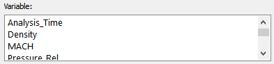
- Math Functions
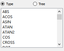
- Math Operators
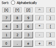
- Evaluate Expression

Math functions use the syntax: function (value or expression). All angle arguments are in radians. For most functions the value can be either a constant, constant per part, scalar, or vector and the result of the function will be of corresponding type. When you select a math function from the list, the function name and the opening "(" appears in the Working Expression for you. However, after defining the argument(s) for the function, you have to manually provide any commas needed and a closing ")".
Note: any calculations involving a vector are done on each component. For
example: GT(vector1,vector2) = (GT(vector1x, vector2x),
GT(vector1y, vector2y), GT(vector1z, vector2z))
The Math functions include the following:
|
Routines which accept argument(s) of type constant, scalar, or vector and produce the corresponding type of result: (function works on each component of a vector) |
|
|
ABS (constant) absolute value = constant or (scalar) scalar or (vector) vector |
ACOS (constant) arccosine = radian constant or (scalar) radian scalar or (vector) radian vector |
|
ASIN (constant) arcsine = radian constant or (scalar) radian scalar or (vector) radian vector |
ATAN (constant) arctangent = radian constant or (scalar) radian scalar or (vector) radian vector |
|
ATAN2(y, x) calculates ATAN(y/x) where the signs of both variables are used to determine the quadrant of the result. Returns the result in radians which is between -PI and PI (inclusive). So: ATAN2(constant, constant) = radian constant or (constant, scalar) = radian scalar or (constant, vector) = radian vector or (scalar, scalar) = radian scalar or (scalar, vector) = radian vector or (vector, vector) = radian vector ATAN2(vector1,vector2) = (ATAN2(vector1x/vector2x), ATAN2(vector1y/vector2y), ATAN2(vector1z/vector2z)) |
|
|
TAN (radian constant) tangent = constant or (radian scalar) scalar or (radian vector) vector |
CROSS (vector, vector) cross product = vector |
|
COS (radian constant) cosine = constant or (radian scalar) scalar or (radian vector) vector |
SIN (radian constant) sine = constant or (radian scalar) scalar or (radian vector) vector |
|
CDF_CHISQU(v,k) evaluates the cumulative Chi-Squared distribution at the value v with k degrees of freedom. CDF_CHISQU(constant, constant) = constant or (constant, scalar) = scalar or (scalar, scalar) = scalar or (scalar, constant) = scalar CDF_CHISQU(v,k) = |
|
|
CDF_F(v, j, k) evaluates the cumulative F distribution at the value v with j and k degrees of freedom. If any input value is a scalar then the result is a scalar. CDF_F(scalar, constant, constant) = scalar or (constant, scalar, constant) = scalar or (constant, constant, scalar) = scalar or (constant, constant, constant) = scalar etc. CDF_F(v, j, k) = |
|
|
CDF_NORM(v) evaluates the cumulative normal distribution at the value v. CDF_NORM(constant) = constant or (scalar) = scalar CDF_NORM(v) = |
|
|
CDF_T(v, k) evaluates the cumulative Student's T distribution at the value v with k degrees of freedom. CDF_T(constant, constant) = constant or (constant, scalar) = scalar or (scalar, scalar) = scalar or (scalar, constant) = scalar CDF_T(v, k) = |
|
|
DOT (vector, vector) dot product = scalar Note: DOT(velocity,velocity) is a scalar not equal to velocity^2 which is a vector.
|
EXP( constant ) e value = constant or ( scalar ) scalar or ( vector ) vector |
|
GT(constant,constant) greater of = constant or (constant,scalar) scalar or (constant,vector) vector or (scalar,scalar) scalar or (scalar,vector) vector or (vector,vector) vector GT(vector1,vector2) = (GT(vector1x, vector2x), GT(vector1y, vector2y), GT(vector1z, vector2z) ) |
|
|
INT(variable) converts all values to signed integers by simply discarding the decimal portion. Note: The decimal portion, FRAC, can be obtained as FRAC = var-INT(var).
|
|
|
LOG( constant ) ln = constant or ( scalar ) scalar or ( vector ) vector |
LOG10( constant ) log 10 = constant or ( scalar ) scalar or ( vector ) vector |
|
LT(constant,constant) lesser of = constant or (constant,scalar) scalar or (constant,vector) vector or (scalar,scalar) scalar or (scalar,vector) vector or (vector,vector) vector LT(vector1,vector2) = (LT(vector1x, vector2x), LT(vector1y, vector2y), LT(vector1z, vector2z) ) |
|
|
MOD(var1,var2) modulo of int(var1) / (int(var2), (that is, the remainder of two integer divisions). or (constant,scalar) scalar or (constant,constant) constant or (scalar,constant) scalar or (scalar,scalar) scalar Note: The first and second values are converted to integers by simply dropping fractional values (no rounding) prior to the integer division. The result (that is, the remainder) is therefore always an integer.
|
|
|
IF_CMP( var,var ) compare the two values and return a -1 or 0, where var can be same as LT above. return value for IF_COMP(a,b): (a < b) returns -1, (a = b) returns 0, (a > b) returns 1 |
IF_EQ( var,var )compare the two values and return a 1 or 0 where var can be same as LT above return value for IF_EQ(a,b): (a = b) returns 1, otherwise returns 0 |
|
IF_LT( var,var )compare the two values and return a 1 or 0 where var can be same as LT above return value for IF_LT(a,b): (a < b) returns 1, otherwise returns 0 |
IF_GT( var,var )compare the two values and return a 1 or 0 where var can be same as LT above return value for IF_GT(a,b): (a > b) returns 1, otherwise returns 0 |
|
PDF_CHISQU(v, k) evaluates the Chi-Squared probability density at the value v with k degrees of freedom. PDF_CHISQU(constant, constant) = constant or (constant, scalar) = scalar or (scalar, scalar) = scalar or (scalar, constant) = scalar PDF_CHISQU(v, k) = |
|
|
PDF_F(v, j, k) evaluates the F probability density at the value v with j and k degrees of freedom. PDF_F(scalar, constant, constant) = scalar or (constant, scalar, constant) = scalar or (constant, constant, scalar) = scalar or (constant, constant, constant) = scalar etc. PDF_F(v, j, k) = |
|
|
PDF_NORM(v) evaluates the normal probability density at the value v. PDF_NORM(constant) = constant or (scalar) = scalar PDF_NORM(v) = |
|
|
PDF_T(v, k) evaluates the Student's T probability density at the value v with k degrees of freedom. PDF_T(constant, constant) = constant or (constant, scalar) = scalar or (scalar, scalar) = scalar or (scalar, constant) = scalar PDF_T(v, k) = |
|
|
RMS (vector) root-mean-square (magnitude) = scalar. RMS(vector) is the same as SQRT(vector[X]*vector[X] + vector[Y]*vector[Y]+vector[Z]*vector[Z]) and the same as SQRT(DOT(vector,vector)) but NOT the same as SQRT(vector^2) |
RND(constant) round to nearest = constant or (scalar) scalar or (vector) vector |
|
LOOKUP (lookup table # (int), scalar) or (lookup table # (int), vector) finds the value of the scalar or vector using the x value in the lookup table and returns the interpolated y value of y. The lookup table x and y values must be defined in advance in the proper case, using EnSight Python. For example, if you define a table number 1,
such that
and the value of the variable myscalar is 0.0, 25.0, 50.0, and 37.5 at elements 1-4 respectively, then the values for myvar will be 0.0, 100.0, 200.0, and 150. at elements 1-4 respectively. Prior to this calculation, create lookup table 1 for this example, with a min and max of 0 and 50 respectively, using EnSight Python, using the following two EnSight Python command lines.
# input values: (table#, xlist, ylist, minx, maxx)
|
SQRT (constant) square root = constant or (scalar) scalar or (vector) vector |
|
UNDEFINED returns the Undefined value. This can be used as a test in IF_EQ(var,UNDEFINED) will return 1 where the variable is undefined and 0 where it is defined. |
|


This on-screen calculator can usually be used in place of typing on your keyboard.
| Button | Function |
|---|---|
| 0 to 9 | number digits |
| . | decimal |
| e | e for exponential notation |
| + | plus operator |
| - | minus operator |
| * | multiplication operator |
| / | division operator |
| ^ | exponentiation operator |
| PI | value for π |
| ( | opening parentheses. For function arguments and general grouping |
| ) | closing parentheses. For function arguments and general grouping |
| [ | opening brackets. For components and node/element numbers |
| ] | closing brackets. For components and node/element numbers |
| [X] | X component |
| [Y] | Y component |
| [Z] | Z component |
(see Create New Variables).