


EnSight includes a number of readers for non-native (non-EnSight) formats. This section includes a description of each of these included readers and includes instruction for their use. Some of the included readers are custom, internal readers, and some of them are written using the standard, User Defined Reader interface.
- 2.3.1. ABAQUS_ODB Reader
- 2.3.2. AIRPAK/ICEPAK Reader
- 2.3.3. AcuSolve Reader
- 2.3.4. Ansys Reader
- 2.3.5. Ansys Fluids Post Reader
- 2.3.6. Autodyn Reader
- 2.3.7. AVUS Reader
- 2.3.8. Barracuda Reader
- 2.3.9. CFF Reader
- 2.3.10. CFX Reader
- 2.3.11. CGNS Reader
- 2.3.12. CGNS-XML Reader
- 2.3.13. CTH Reader
- 2.3.14. Dynamic Visualization Store (DVS) Reader
- 2.3.15. EXODUS II Reader
- 2.3.16. FAST Unstructured Reader
- 2.3.17. FIDAP NEUTRAL Reader
- 2.3.18. FLOW3D-MULTIBLOCK Reader
- 2.3.19. Fluent Direct Reader
- 2.3.20. Fluent_HDF5
- 2.3.21. FORTE
- 2.3.22. LS-DYNA Reader
- 2.3.23. LSTC-LS-DYNA Reader
- 2.3.24. MSC.DYTRAN Reader
- 2.3.25. MSC.MARC Reader
- 2.3.26. NASTRAN OP2 Reader
- 2.3.27. OpenFOAM Reader
- 2.3.28. OVERFLOW Reader
- 2.3.29. PLOT3D Reader
- 2.3.30. RADIOSS Reader
- 2.3.31. Polyflow Classic Reader
- 2.3.32. Rocky Reader
- 2.3.33. Silo Reader
- 2.3.34. Software Cradle FLD Reader
- 2.3.35. STL Reader
- 2.3.36. Synthetic Reader
- 2.3.37. Tecplot Reader
- 2.3.38. Vectis Reader
- 2.3.39. VTK Reader
- 2.3.40. XDMF 2.0 Reader
- 2.3.41. XDMF 3.0 Reader
Note: The following readers are no longer supported and have been removed as of EnSight 2023 R2. To access these readers, you must use an EnSight version prior to 2023 R2:
Converge_Input
FRPR
Inventor
MSC.Marc – Legacy
Nastran Input Deck
SDRC_Ideas
User Defined Reader Description
A user defined reader capability is included in EnSight which allows otherwise unsupported structured or unstructured data to be read. In other words, the user can create their own data readers. Each user defined reader utilizes a dynamic shared library produced by the user. Once produced, these readers show up in the list of data formats in File → Open... just like the included readers.
User Defined Reader Implementation
The readers are produced by creating the routines documented in the user-defined API. Three versions of the user defined API are available The 1.0 API (which has been available since EnSight version 6) was designed to be friendly to those producing it, but requires more manipulation internally by EnSight and accordingly requires more memory and processing time. The 2.0 API (starting with EnSight 7.2) was designed with efficiency in mind. It requires that all data be provided on a part basis, and as such lends itself closely to the EnSight Gold type format. A few of the advantages of the 2.0 API (Now at version 2.08) are:
Less memory, more efficient, and faster - as indicated above.
Model extents can be provided directly, such that EnSight need not read all the coordinate data at load time.
Tensor and complex variables are supported
Exit routine provided, for cleanup operations at close of EnSight.
Geometry and variables can be provided on different time lines (timesets).
If your data format already provides boundary shell information, you can use it instead of the border representation that EnSight would compute.
Ghost cells (for both structured and unstructured data) are supported
User specified node and/or element ids for structured parts are supported
Material handling is supported
Nsided and Nfaced elements are supported
Structured ranges can be specified
Filtered elements are supported
Material Species is supported
Rigid Body values can be supplied from the reader.
Reader can be allowed to deal with block min, max, and stride within itself - instead of having EnSight deal with it.
A 3.0 reader API is available in EnSight 9. The 3.0 API aims to provide the flexibility of both of the previous versions while simplifying the reader development processes. Contact Ansys for more information on this API.
Creating Your Own Custom User Defined Reader
The process for creating and using a user-defined reader is explained in detail in the Ansys EnSight Interface Manual. Samples, source code, makefiles, etc can be found in the following location and its subdirectories:
On the install media: /CDROM/ensight251/src/readers
In an installation directory: $CEI/ensight251/src/readers
Start EnSight (or EnSight server) with the command line option
(-readerdbg), for a step-by-step echo of reader loading progress (see Command Line Start-up Options).
ensight -readerdbg
The actual working user defined readers included in the EnSight distribution may vary by hardware platform.
The following topics are included in this section:
Because the reader is dependent upon the ABAQUS libraries, this reader is only available for platforms supported by ABAQUS.
The reader is available in the following directory:
$CEI\ensight251\machines\win64\lib_readers\udr_abaqus
The ABAQUS ODB reader is the recommended method of importing ABAQUS data into EnSight.
Simple Interface Data Load
Load your geometry/results file (typically named with a suffix .odb) using the Simple Interface method.
Advanced Interface Data Load
Load your geometry/result files (typically named with a suffix .odb) using the Advanced Interface method.
|
Data Tab | |
| Format |
Use the ABAQUS_ODB format. |
| Set geometry |
Select the geometry file (typically .odb) and click this button |
| Set results |
Not used |
|
Format Options Tab | |
| Set measured |
Select the measured file and click this button. |
| Reader GUI |
User controls as shown below are available:
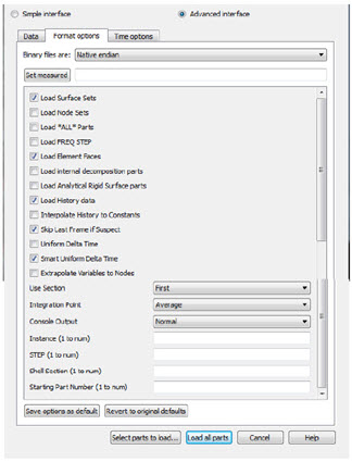 |
| Load Surface Sets |
Toggle ON (default) to load all Surface Sets |
| Load Node Sets |
Toggle ON to load all Node Sets (default OFF). |
| Load "*All*" Parts |
Often, ABAQUS parts that are simply the global element matrix are redundant (for example, E_ALL contains all elements). Toggle OFF (default) to skip loading Parts with all in their name, saving memory and time. |
| Load Freq Step |
Often, ABAQUS will include multiple steps in an .odb file and the one desired is the modal analysis. Toggle this ON to skip all other steps loading only the frequency step (Default is OFF). If multiple frequencies, then each EnSight timestep now becomes a different frequency. |
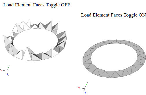
| Load Element Faces |
Toggle ON to convert Surface Sets with 3D elements with Face Sets into 2D elements using face specifications where indicated by the ABAQUS dataset. (default ON). |
| Load internal decomposition parts |
Toggle ON to load internal decomposition sets (that show the parallel decomposition of the ABAQUS solver) as EnSight parts.(default OFF). |
| Load Analytical Rigid Surface parts |
Toggle ON to load rigid surface parts as transient, rigid
line segments that can be extruded in 3 dimensions. This can be done using a
python script. Contact |
| Load History Data |
Toggle ON to load History data which will load either as constants or as queries over time (default ON). Some datasets contain history data at extremely high sample rates with large number of xy data pairs. EnSight is not structured to be able to handle large numbers of queries with a large number of data pairs, and will abort the loading of history data if it encounters a data pair with more than 3000 samples. The reader will output a warning that it has aborted the history data read and that you can override this number; set the environmental variable on the server as follows: set ENSIGHT_READER_MAX_QUERY_PAIRS to the maximum number of pairs that you wish to allow and restart EnSight. |
| Interpolate History to Constants |
History data is typically input to EnSight as queries (curves). EnSight has the ability to use constant (single values at each timestep) in ways that are not available to queries. If this is ON then History variables will be interpolated as EnSight Constants (if extrapolation is not necessary). If OFF then History variables will be read in as constants only if there is an exact one to one match of time values for each EnSight timestep (Default OFF). |
| Skip Last Frame if Suspect |
If the ABAQUS solver crashes, it can dump out a variety of variable values for the last FRAME in the ODB file that may be spurious. Toggle this ON (default) to check the last FRAME in a STEP for an increase in the number of variables and, if so, skip it. Toggle this OFF to ignore warning signs and load the data from the last frame. If suspect values are found in the last FRAME, then NAN checking of each variable value is turned on, with NANs returned as zero (Default ON). |
| Smart Uniform Delta Time |
Some ABAQUS STEPs have frame values that are constant (and very small). Frame values are used by EnSight for time steps and therefore from this type of STEP are not monotonically increasing in time and EnSight will skip these timesteps. Toggle this ON, and EnSight will automatically convert time values from selected ABAQUS STEPs into using a delta time of 1.0 (default is ON). Because EnSight is automatically changing the timestep
values, this will only be done to selected ABAQUS STEPs (more may be added
over time). The current list of these includes only one ABAQUS STEP:
*STEP PERTURBATION, *STATIC. As new STEPs are encountered
they may be added to this list and documented. If a new STEP is encountered with
non monotonically changing time values that should be added to this list, please
contact Because this changes the ODB time values, this Toggle was added to allow you to turn this off and use the frame values as the time values in EnSight. |
| Uniform Delta Time |
Some ABAQUS STEPs have Frame values that are constant (and very small). Frame values are converted to float values and are used by EnSight for time steps. Time values may therefore become not monotonically increasing in time and then EnSight will skip these timesteps. Toggle this ON, and EnSight will automatically convert ALL ABAQUS Frame time values from all ABAQUS STEPs into using a uniform delta time of 1.0. Because this changes the ABAQUS ODB time values for ALL of the ABAQUS STEPs it is by default OFF. |
| NaN Check | The ABAQUS ODB solution data is converted in the ODB API from double precision EnSight single precision, float. The default is to check all floating point values and to print a warning in the message window if there is a problem. This conversion of the raw data sometimes results in Not A Number values or denormalized floats (almost NaNs which should not be used in further calculations). If you get a warning in the message box that you have denormalized floats, try checking the message window for Extrapolate Variables to Nodes (see below). |
| Extrapolate Variables to Nodes |
Variable values are extrapolated to the nodes using the ABAQUS internal API from each element's internal integration points to the nodes from each element. The reader then does a simple average of the nodal values from each element. This has been demonstrated to give the same results as ABAQUS CAE. Because the simple averaging is done within the ABAQUS API, it has been seen to eliminate some of the NAN issues described above. |
| Load Warn parts |
The ODB dataset includes subset parts that contain exist to Warn the user of element or variable anomalies. Often this can result in an excessive number of parts in the EnSight part list. Toggle ON to load parts starting with Warn* (default) and OFF to skip these parts. It is recommended that you skip these parts if EnSight is slow to load data or activate variables due to a large number of parts. |
| Use Section |
Shell elements include variable data for each section. This reader allows the use of the First (default) or the Last section. |
| Integration Point |
Shell elements include variable data for each of several integration points. Choose max, min or average (default). |
| Console Output |
Normal - Informational and error output to the console. Verbose - Detailed informational and error output to the console. Debug - Step by step progress through the reader with detail numerical output for results to the console. None - No console output |
| Instance |
Choose an instance ( |
| Step |
Choose a step ( |
| Shell Section |
Which shell section to use ( |
| Starting Part Number (1 to num) |
Which part to begin loading (default is empty which is the first part). |
| Ending Part Number (1 to num) |
Which part to end loading (default is empty, which is last part). |
Older Version ODB Files
The EnSight ODB reader will be able to read .odb files from 6.1 to the current version using the upgrade utility. If upgrade is needed, the original ODB file is read in and left unchanged, while an upgraded copy is automatically written in the same directory (user must have write permission in this directory). UPGRADE_6_* is added to end of filename prefix, where the * is the current library version, for example UPGRADE_6_14 for ODB library version 6.14. The current library version can be seen in the file open dialog under the Data tab, when you choose the ABAQUS_ODB reader in the reader selection pulldown in advanced mode. The reader version will appear just below the pulldown in the reader description box.
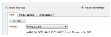
The first numbers (for example, v2018) indicate the API (which corresponds to solver version 2018) as shown in the above figure.
Shell Elements
In ABAQUS, many shell elements have sections and integration points. Sections are regions such as top or bottom of a beam. Integration points are specified locations on the sections. In contrast, EnSight elements have only one value per element. So it is necessary to have a mapping scheme between the multiple element values in ABAQUS and the single EnSight elemental value. Choose the Format options tab in the data reader dialog to change the mapping of shell elemental variable data from ABAQUS to EnSight.
Integration Point pulldown allows the choice of the max, min or average (default) of the integration points at a shell element to use as the EnSight variable value.
The Use Section pulldown allows the choice of the first (default) or last section at a shell element to use as the EnSight variable value.
To enter in a section number of your choosing (if there are more than
two), simply enter a value (1 to number of sections) into the
Section field. Entering a value into this field (default is empty)
supersedes the choice in the pulldown.
Modal Data
Sometimes the analysis will have transient/static STEPs along with FREQUENCY STEPS. EnSight can handle either transient/static or frequency data, so by default, with mixed data, the FREQUENCY STEPs are skipped, and only the transient/static STEPs are loaded.
If you want only the modal data, toggle ON the Load FREQ STEP toggle, and the reader will use the first modal frequency STEP. Also, if, for example, you know the modal FREQUENCY STEP, you can also select the step number by entering it in the STEP (1 to num) field
Once your modal data is loaded, to visualize the modal displacement, select the part(s) of interest, and displace by the displacement vector, U. Each modal frequency is loaded in as a separate EnSight timestep, so step through EnSight "times" to step through the frequencies. Similarly you can view the modal velocity, V or the acceleration, A.
Each modal frequency is stored as a single value for a given EnSight timestep. You can access these EnSight constants as follows:
Modal Frequencies (single value constants) are stored in the constant, single value variable, H_EIGFREQ. Modal Eigen values (single value constants) are stored in the single value variable H_EIGVAL.
Note: For any given mode, H_EIGVAL is (2 * PI * H_EIGFREQ)^2. These values are helpful, for example, to display the frequency as an annotation that updates when the timestep is updated.
Modal Participation Factors (single value constants) are as follows:
H_PF1 - Participation factor, x-component
H_PF2 - Participation factor, y-component
H_PF3 - Participation factor, z-component
H_PF4 - Participation factor, x-rotation
H_PF5 - Participation factor, y-rotation
H_PF6 - Participation factor, z-rotation
Analytical Rigid Surfaces
ABAQUS ODB data includes three Analytical Rigid Segments that do not have variable data, do not deform, and only move rigidly in translation or rotation that are of type
REVOLUTION - A rigid segment rotated about a point
CYLINDER - A rigid segment translated in a given direction
BSURF - A line segment used in 2D analysis
These parts are read in as line segments if the user toggles ON the Load Analytical Rigid Surface parts toggle in the Format options tab in the data reader dialog for the ABAQUS_ODB reader. These segments are translated and rotated independently of the rest of the ABAQUS model using U and UR of the reference node using EnSight's rigid body capability. These segments will displace and rotate automatically according to their proscribed motion in the ODB file using EnSight's rigid body implementation, so U and UR cannot be applied to the ARS segments, and all variables are disabled for ARS segments. Conversely, you cannot undisplace an Analytical Rigid Segment. To get other parts to match the automatic displacements / rotations of the ARS, you will need to turn on displacements of your normal parts.
Analytical Rigid Surfaces Manual Creation
In order to turn the Analytical Rigid Segment into an Analytical Rigid Surface, you can use EnSight's Extrude function. If the segment part has REV in the name, then you'll want to rotate, and you can toggle ON to rotate about a part centroid, and choose the part id of the rigid reference node corresponding to this ARS part, pick the rotational degrees and the axis, and click Create to construct the extruded rotational surface.
Note: Since the ARS segment is moving automatically, and the rigid reference node is not moving automatically, if you want to track the actual motion of the rigid revolution part, you will want to turn on displacements for the Rigid Reference point part, then toggle on Displace Computationally so that the rigid reference node displacements are used in the calculations. If the segment part has CYL in the name, then you'll want to extrude the part in a given direction, with a total translation. This extruded part should automatically move correctly without any other steps. Since the EnSight extrude function allows you to select a part centroid (such as a rigid reference node) for the origin, the roller can move around as the reference point moves. However since the extrude function only allows the choosing of a static axis direction, the axis of the extruded part cannot change over time.
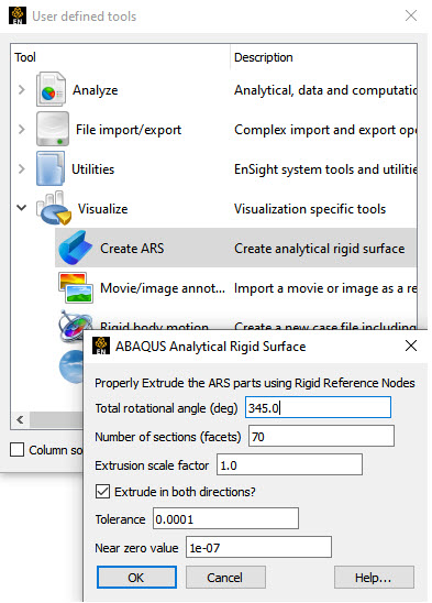
Analytical Rigid Surfaces Automatic Creation Using Python Tool
Should you want all of this done for you automatically, there is a python tool included with EnSight that will automatically create all of your Analytical Rigid Surfaces. As shown in the figure below, simply click the tools icon at the top and choose the Create ARS icon under the Visualize folder. Simply fill in the graphical user interface and it will turn on computational displacements of the rigid reference nodes automatically and just create the rigid reference surfaces as expected.

If the default behavior of the reader is unexpected (that is, no parts loaded, too few timesteps loaded, or variables not available) then reload the .odb file and select the Format options tab and choose Console Output: Debug. Then take a look at the output in your server console.
Missing Parts
Are you missing parts? By default, EnSight does not load the
nodesets. Toggle this ON to load the nodal parts. By default, EnSight does not load parts
whose names containing ALL or All because these are often duplicate parts that double the
required memory and slow down the operation of the reader. Toggle ON the Load
*all* toggle to load these parts. If you have no parts loaded, take a careful
look at the console output (see below) and notice that all of the nodesets are skipped, as
is the ALL_ELEMENTS part, therefore you have no parts
loaded.
-----------------------------------------------------------
              EnSight ABAQUS Parts
              Total num Instances 1
              Total num nodes 936
              Total num elements 625
    Choose 'Format options' tab in data reader dialog
    To load or skip node or surface sets:
        Toggle OFF 'Load Surface Sets'
        Toggle OFF 'Load Node Sets'
    To load or skip sets with ALL in their name:
        Toggle OFF 'Load *ALL* Parts'
-----------------------------------------------------------------------------------
    ABQ Ens Part Instance & Type Number Status
    Num Num Name Elements
------- ------ --------------- --------- -------
1. 1. ALL NODES Assm 0 Nodeset 1 SKIPPED
2. 1. ALL NODES Assm 1 Nodeset 936 SKIPPED
3. 1. ASSEMBLY_CONSTRAINT-1_NODES Assm 1 Nodeset 36 SKIPPED
4. 1. ASSEMBLY_CONSTRAINT-1_POINT Assm 0 Nodeset 1 SKIPPED
5. 1. ALL ELEMENTS Assm 1 Elemset 625 SKIPPED
-----------------------------------------------------------
Number of regular ABAQUS parts = 5
Number of Analytical Rigid Surface parts = 0
Total number of Abaqus parts = 5
Total number of EnSight parts = 0
-----------------------------------------------------------
-----------------------------------------------------------
Missing Timesteps
Are you missing timesteps? Each ABAQUS FRAME is an EnSight timestep. If the change in time between two successive frames is too small to represent as a float value, then EnSight will skip it.
ABAQUS data is loaded in STEPs. Since EnSight has only timesteps (transient) or one timestep (static) there is a bit of mapping that goes on to read in an odb dataset.
ABAQUS STEPs of type *STEP PERTURBATION, *STATIC" STEP are now loaded with their timesteps incremented by 1.0. The Toggle Smart Uniform Delta Time has been added to turn this off and use the frame values (which are 2E-16). This is ON by default.
Important: This automatically changes timestep time values. Since other STEPs may also have very small delta time, the Toggle Uniform Delta Time is included so that the time values can be made to increment by 1.0 for ALL STEPs of the ODB data. (default OFF).
To pick a given ABAQUS STEP, for example, STEP 4 (1- based),
simply enter 4 into the STEP (1 to num)
field.
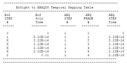
Here is the details on the load steps and times and is consistent with ABAQUS handling of .fil.
ABAQUS STEP is an EnSight Case. Each ABAQUS FRAME is a time increment to the final STEP value. The EnSight total time is a unique cumulative value for each EnSight timestep that is monotonically increasing.
Each odb STEP is like a sequential, but separate analysis.
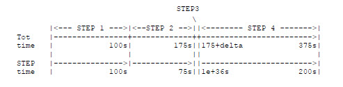
The ODB API reports data by STEP with each step having a series of FRAMES each representing an EnSight timestep. EnSight use the ABAQUS TOTAL TIME as our Solution Time. Apparently, an ABAQUS user can look at their status file and know what TOTAL TIME relates to the STEP.
If we had a file with 3 ABAQUS STEPS, and 5 increments per step:
Notice the ABAQUS odb details in the left columns and the resulting EnSight mapping on the right. The X is a timestep that is excluded from EnSight because there is no time change from the previous step.
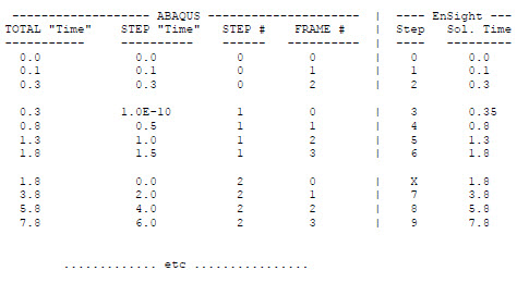
Therefore, if you wanted to look at:
The 1st load case (STEP 0):
Look at Ensight times
0 - 0.3 or EnSight
steps 0 - 2
The 2nd load case (STEP 1):
Look at Ensight times
0.35 - 1.8 or
EnSight steps 3 - 6
The 3rd load case (STEP 2):
Look at Ensight times
1.8 - 7.8 or
EnSight steps 6 - 9
Note: Times that have no total time increment are dropped from EnSight.
Times that have an extremely small increment (for example, 1E-10) are incremented larger so that the time can be represented as a float.
For example, when you see the
X in the left hand column below, this timestep is
skipped because you can see that the increment is essentially zero. A number of steps
are skipped below for that reason.
Missing Variables
When you choose Console Output Debug, you
can see the list of variables in the console output and that some of the variables are
skipped. Skipped variables include the _MAG variables, which are vector
magnitude that EnSight auto-calculates for vector variables from the components. You can
see that some of the contact variables, which are part-specific are combined into one,
single value.
Odd Part Shapes
When you read in your parts if the Surface Set parts seem to have full elements showing and you only want the selected faces of the elements to be used to form your parts, then reload your data and choose Load Element Faces in the Format options tab of the Data Reader dialog.
See Read Data
The following topics are included in this section:
The current Fluent Direct Reader also reads Ansys Airpak and Ansys Icepak data. The Fluent Direct reader typically loads a Fluent case (.cas) file and the matching data (.dat) file. However, Ansys Airpak and Ansys Icepak writes out a .fdat file which doesn't automatically get recognized by the EnSight Fluent reader and some extra understanding (and sometimes user-intervention) is necessary as described below.
See the following files for the latest information on the Fluent reader.
$CEI/ensight251/src/readers/fluent/README.txt
The comments that follow are for the current Fluent reader. The reader loads ASCII, binary single precision, or binary double precision. The files can be uncompressed or compressed using gzip.
Data File Description
Icepak can generate files: filename.cas, filename.dat just like Fluent, but also if the analysis uses a nonconformal mesh (not available in Fluent) then there will be filename.fdat, and filename.nc.cas files. The filename.nc.cas is a nonconformal mesh geometry and its matching results file is the filename.fdat file.
Simple Interface Data Load
Load your geometry file (typically named with a suffix .cas ) using the Simple Interface method. EnSight will automatically load the matching .dat file. However, if you want to load the filename.nc.cas data file and its corresponding filename.fdat file, then you will either need to rename it to match exactly and have the .dat extension (filename.nc.dat), or go to the advanced data load.
See Read Data and Fluent Direct Reader.
The following topics are included in this section:
Description
This reader from AcuSim will read results from Acusolve. Select the .log file from the simple or advanced interface.
File → Open...
The File Selection dialog is used to specify which files you wish to read.
File → Open...
Simple Interface Data Load
Load your AcuSolve .log file using the Simple Interface method.
Advanced Interface Data Load
Load your AcuSolve .log file using the Advanced Interface method.
|
Data Tab | |
| Format |
Use the AcuSolve format. |
| Set file |
This field contains the first file name. For the first file you should choose a file with extension .log. Clicking button inserts file name shown into the field. Loading the .log file will load all both geometry and results. |
|
Format Options Tab | |
| Set measured |
Select the measured file and click this button. |
|
Other Options |
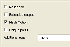 |
| Reset time |
When toggle is on, time begins at 0.0 (default is off). |
| Extended output |
When toggle is on, console output will be verbose (default is off). |
| Mesh Motion |
When toggle is on, moving meshes are visible (default is on). |
| Unique parts |
When toggle is on, a unique set of surfaces is shown in the part list (default is off). |
| Additional runs |
Enter the comma separated list of runs
( |
Note: There is an older AcuSolve (v10 api) reader available from AcuSim.
The following topics are included in this section:
Three Ansys Readers
There are three Ansys readers available in EnSight: two older, unsupported legacy readers and the supported Ansys Results. Long-term, Ansys Results is the reader of choice. This reader should read the latest Ansys results as well as older versions. The other two, legacy readers will not show up in the reader list by default and will not be documented in this manual.
Legacy Reader Visibility Flag
The older readers, by default, are not loaded into the list of available readers, and are not discussed in the remainder of this document. In the unlikely event you need to enable these readers, go into the Menu, Edit → Preferences and click on Data and toggle on the reader visibility flag. The legacy reader documentation is found in $CEI/ensight251/src/readers/ansys/README and is not included here.
Ansys Results Reader
The Ansys Results reader supports scalar, vector and tensor variables, including the capability to compute several common scalar variables derived from tensors (such as the common failure theories) as well as local element result components (such as axial stress in truss elements) when such element results are available. Additionally, there is some control over the creation of variables from element-based results. For example, they can be averaged to the nodes (with or without geometry weighting) if desired. See the format options below for more details.
Results are always presented in the global coordinate system. Therefore, any results in local coordinate systems, or in non-cartesian coordinate systems are transformed as needed into the model system.
For shell elements that have multiple layers (sections), you can choose the section that will be used. Additionally, you can choose to have a different variable be created for each section. See format options below for more details.
You can control how parts are created. Parts can be created according to the part id, the property id, or the material id.
Ansys has added a new data compression algorithm (sparsification) to the output of Ansys Mechanical that has caused read failures in the EnSight Ansys mechanical reader when, for example attempting to open some .rst files. This reader now supports datasets utilizing this compression algorithm.
Simple Interface Data Load
Load your geometry/results file (typically named with a suffix .rst) using the Simple Interface method.
Advanced Interface Data Load
Load your geometry/result files (typically named with a suffix .rst) using the Advanced Interface method.
|
Data Tab |
|
|
Format |
Use the Ansys Results format. |
|
Set file (or results) |
Select the geometry/results file (typically .rst, .rth, or .rmg) and click this button |
|
Format Options Tab |
|
|
Set measured |
Select the measured file and click this button. |
|
Other Options |
 |
|
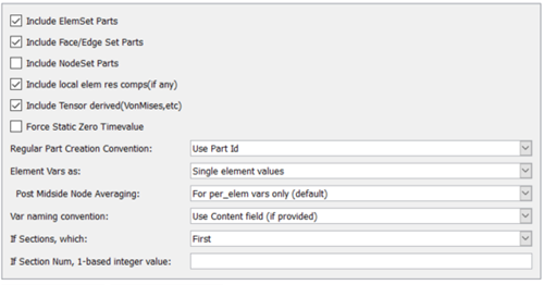
Include any Element sets defined. These are sets of full elements which are generally some logical subset of the total number of elements. Default is on. |
|
|
Include Face/Edge Parts |
Include any Face or Edge sets defined. These are some logical set of particular faces and/or edges of full elements. Default is off. |
|
Include NodeSet Parts |
Include any Node sets defined. These are generally the subset of nodes needed for the Element, Face, or Edge sets above. As such, they are generally not needed as separate parts, but can be created if desired. Default is off. |
|
Include local elem res comps (if any) |
Include the local stresses components, etc that are in the element's local system. A simple example is a bar (such as a truss element), which only has tension or compression in the element's axial orientation. Such an element would have an axial stress variable. Other elements would have appropriate result component variables. Default is on |
|
Include Tensor derived (VonMises, etc.) |
For tensor results, calculate scalars from
the following derived results (principal stress/strains, and common failure theories):
Mean Equal Direct VonMises Min Principal Octahedral Mid Principal
                Intensity Max Principal Max Shear
By default, all 9 of these will be derived. You can control which are created by this toggle, with an environment variable. Namely,
or any legal combination. example: for VonMises and Max Shear only, use 18. Default is on. |
|
Force Static Zero Timevalue |
Make the RST file return single time step for static data and apply Displacements by default. |
|
Regular Part Creation Convention |
Parts will be created according to the following: Use Part Id - Part Id (this is the default) Use Property Id - Property Id Use Material Id - Material Id |
|
Var naming convention |
Use Content Field (if provided) - Variable names will be what is in the Content field, if provided. If not provided, they will be the VKI dataset name. This is the default. Use VKI dataset name Variable names will be the VKI variable dataset name (which are reasonably descriptive). |
|
Element Vars as |
Single element values - Element results (whether centroidal or
element nodal) will be presented as a single value per element. Therefore will be
Averaged to node values - Element results (whether centroidal
or element nodal) will be averaged to the nodes without using geometry weighting.
Therefore will be Geom weighted average to node values - Element results (whether
centroidal or element nodal) will be averaged to the nodes using geometry weighting.
Therefore will be Ave to node values <by parts> - Element results (whether
centroidal or element nodal) will be averaged to the nodes without using geometry
weighting. Therefore will be Geom weighted ave to node <by parts> - Element results
(whether centroidal or element nodal) will be averaged to the nodes using geometry
weighting. Therefore will be |
|
Post Midside Node Averaging |
Average Off - No midside node averaging. For per_elem vars only (default) - Midside node averaging of element results only.
For per_elemnode only - Midside node averaging of element node
results only. These variables will have
Both - Both |
|
If Sections, which: |
Which section will be used to create the variable First - The first section will be used (this is the default) Last - The last section will be used Section Num (below) - The section number entered in the field below will be used Separate Vars per Section - A separate variable will be created for each section. |
|
If Section Num, 1-based integer value: |
If the previous option is chosen to be Section Num, then the value in this field is the 1-based section number to use to create the variable. |
Note: EnSight 2023 R1 has an updated Ansys Results reader. As part of this update and compliance with changes in format and understanding, there are changes to some of the variable names, as well as variables omitted (by design) with the new reader. Unfortunately, due to the nature of the change, and the variability of that change, the entire list of variable names changed or omitted from this version of the reader cannot be explicitly listed.
Example 2.1: Variable Name Change
Vector Contact_Displacement_el is no longer available.
However Contact__Slip_Displacement_el is available as a
scalar. (magnitude of that vector)
Element_Nodal_Flux_el is now
Element_Nodal_Heat_Flux_el
Limitations
EnSight is designed to post process results independent of any solver. As such EnSight lacks tools and tight integration with the Ansys Mechanical solver that are necessary for some Mechanical Analyses such as the following:
Mechanical Failure
Eigenvalue Buckling
Fatigue, Harmonic Acoustic/Response
Modal
Modal Acoustics
Random Vibration
Response Spectrum
Data files from these analyses may read fine into EnSight but they will be lacking the necessary variables and/or the tools required for accurate, timely post-processing of these analyses.
The following topics are included in this section:
Ansys Common Fluids Format (CFF) Post, is intended to be a post processing format whose variable values are the same as those shown in the native solver post processor. In EnSight, the Ansys Fluids Post reader was written to read Ansys Common Fluids Format files written 2020 R2 onwards, which includes the following: (the project file (.flprj) which will load the .cas.post and .dat.post files) by Fluent, (the project file (.flprj) which will load the .cas.cff and .dat.cff files) by CFX, (.cas.fsp and .dat.fsp) by FENSAP and (.cas.poly and .dat.poly) by Polyflow Classic. This reader uses the Ansys CFF SDK (R25.1) to read all of the information from the .cas.(post/cff/fsp/poly) and .dat.(post/cff/fsp/poly) files. This reader relies entirely on CFF SDK to provide necessary information to create parts and variables. The Project file is required to determine the correct time value for transient solutions. In addition, project file contains flags which are used by reader to determine about changing connectivity and coordinates (and is therefore strongly suggested for transient runs) if it is available (FENSAP and Polyflow Classic do not yet export the project file).
Note: Duplicate part names are not supported in Ansys Fluids Post reader. By default, Fluent assigns zone names to zone surfaces. For the reader to load them correctly, you need to assign a different name to the zone surface if both volume parts and surface parts are present in a Fluent exported post file.
Simple Interface Data
Load Fluent exported .cas.post and .dat.post files using the project file (.flprj) if it is available. You should provide the project file(.flprj) if it is available, otherwise .cas.post file, and EnSight will attempt to read similarly named .dat.post files as well. EnSight will similarly attempt to load CFX exported (.cas/.dat).cff (via the project file), FENSAP exported (.cas/.dat).fsp or Polyflow Classic (.cas/.dat).poly files.
Advanced Interface Data
Load Fluent geometry and result information (typically named with suffix .cas.(post/cff/fsp/poly) and .dat.(post/cff/fsp/poly) respectively) which has been exported from Fluent/CFX/FENSAP/Polyflow Classic 2020R2 or later.
.cas.post
If the project file (.flprj) is available, select and click , otherwise if the project file is unavailable, select the geometry file (typically .cas.(post/cff/fsp/poly) and click this button. For transient geometry data, if the project file is unavailable, use a single asterisk to replace the step or time number (*.cas.(post/cff/fsp/poly).
.dat.post
Select the results file (typically .dat.(post/cff/fsp/poly) and click this button. For transient variable data, use a single asterisk to replace the step or time number (*.dat.(post/cff/fsp/poly). There is no need to select result file(s) if project file is provided as mentioned above.
Table 2.1:
| Data Tab | |
| Format |
To use the reader, choose format. |
|
| Select the geometry file (typically .cas.(post/cff/fsp) and click this button. For transient geometry data, use a single asterisk to replace the step or time number (*.cas.(post/cff/fsp). If project file (.flprj) is available, select and click on |
| Select the results file (typically .dat.(post/cff/fsp) and click this button. For transient variable data, use a single asterisk to replace the step or time number (*.dat.(post/cff/fsp). There is no need to select result file(s) if project file is provided as mentioned above. | |
|
Format Options tab | |
| Other Options |  |
| Console Output | // adjusts the output information to assist in debugging issues. |
| Maximum number coprocessing timesteps (default 0, off) |
This allows EnSight to post process a running, transient solution (e.g. coprocess), checking for new cas.(post/cff/fsp) and dat.(post/cff/fsp) (1 per timestep) as the solution proceeds and adding timesteps to the time dialog as they are encountered. If non-zero, this specifies the maximum number of possible timesteps that will be written out during this solution. This is useful to monitor a running solution or to begin post processing a long run without waiting for it to finish. |
Caveats
CFF provides a variable map file for Fluent and FENSAP which is used to assign variable name and its unit. CFX (cas.cff and dat.cff) contains all necessary information to assign correct variable name and unit to it. If you find incorrect variable name or assigned unit please report this issue.
Units are not yet available through CFF API in .cas.post/.dat.post.
Time values for transient simulations are only available if you specify the Fluent Project File (.flprj). If you do not specify this file correctly, EnSight will assign time values as integers equal to timestep (this will not work for Pathlines).
Case Constant variables (for example,
PRESSURE_REForTEMPERATURE_REF) which are available through the Fluent_HDF5 restart (.cas.h5/.dat.h5) reader are not yet supported in .cas.post/.dat.post format process. For more information, see CAS.H5 Constants under Fluent_HDF5.Write permission is required for the directory containing .cas.(post/cff/fsp)/.dat.(post/cff/fsp) files. The CFF API requires write access to the directory containing the .cas.(post/cff/fsp)/.dat.(post/cff/fsp) file. You must ensure that write permission is available.
Variable map file provided by CFF for Fluent and FENSAP contains information to create vector variable which is used to create vector variables. Additionally, you can select the three components in the variable object list and right-click to make into a vector.
Gradients for variables may be zero, or reported incorrectly in the .dat.post file. This is a limitation in Fluent's API.
Variable values for
wall-onlyvariables will be given as zero fornon-wallparts. This adversely effects the default palette range and calculations. You will need to adjust palette and calculations based on wall-only parts forwall-onlyvariables.All variables are given as nodal variables (except the
Overset
                cell
variable used to filter out overset cells). Cell-centric variables (likeCell_Volume, orCell Face Area) are averaged when reported as nodal. You should be aware that this will impact calculations where cell-centric variables are utilized.Overset cells are automatically filtered out using the overset cell variable.
Reader only accepts .cas.(post/cff/fsp) and .dat.(post/cff/fsp) files exported from Fluent version 2020R2 or later.
This data transfer mechanism does not yet handle discrete particle data (DPM). If you are attempting to utilize DPM visualization, you will need to utilize the EnSight Gold Case export mechanism.
The following topics are included in this section:
Description
Reads a series of .adres files as a transient solution. Simply select one of the .adres files and the sequence will be detected. Requires that the .adres_base files exists in the same directory. Supported only on Windows.
File → Open...
The File Selection dialog is used to specify which files you wish to read.
File → Open...
Simple Interface Data Load
Load your Autodyn .adres file using the Simple Interface method.
Advanced Interface Data Load
Load your Autodyn .adres file using the Advanced Interface method.
|
Data Tab |
|
|
Format |
Use the Autodyn format. |
|
Set file |
This field contains the first file name. For the first file you should choose a file with extension .adres. Clicking button inserts file name shown into the field. Loading any .adres file will load all .adres files in the directory which includes both geometry and results. |
|
Format Options Tab |
|
|
Set measured |
Select the measured file and click this button. |
|
Other Options |
 |
|
Include any Element sets defined. These are sets of full elements which are generally some logical subset of the total number of elements. Default is on. |
|
|
Include Face/Edge Parts |
Include any Face or Edge sets defined. These are some logical set of particular faces and/or edges of full elements. Default is off. |
|
Include NodeSet Parts |
Include any Node sets defined. These are generally the subset of nodes needed for the Element, Face, or Edge sets above. As such, they are generally not needed as separate parts, but can be created if desired. Default is off. |
|
Include local elem res comps (if any) |
Include the local stresses components, etc that are in the element's local system. A simple example is a bar (such as a truss element), which only has tension or compression in the element's axial orientation. Such an element would have an axial stress variable. Other elements would have appropriate result component variables. Default is on. |
|
Include Tensor derived (VonMises, etc.) |
For tensor results, calculate scalars from the following derived results (principal stress/strains, and common failure theories): Mean Equal Direct VonMises Min Principal Octahedral Mid Principal
Intensity Max Principal Max Shear
By default, all 9 of these will be derived. You can control which are created by this toggle, with an environment variable. Namely, setenv ENSIGHT_VKI_DERIVED_FROM_TENSOR_FLAG n where n = 1 for Mean only 2
for VonMises only 4 for Octahedral only 8 for Intensity only 16 for Max Shear only
32 for Equal Direct only 64 for Min Principal only 128 for Mid Principal only 256
for Max Principal only 512 for all
or any legal combination. example: for VonMises and Max Shear only, use 18. Default is off. |
|
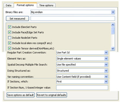
Regular Part Creation Convention |
Parts will be created according to the following: Use Part Id - Part Id (this is the default) Use Property Id - Property Id Use Material Id - Material Id |
|
Var naming convention |
Use Content Field (if provided) - Variable names will be what is in the Content field, if provided. If not provided, they will be the VKI dataset name. This is the default. Use VKI dataset name Variable names will be the VKI variable dataset name (which are reasonably descriptive). |
|
Element Vars as |
Single element values - Element results (whether centroidal or element nodal) will be presented as a single value per element. Therefore will be per_elem variables in EnSight. This is the default. Averaged to node values - Element results (whether centroidal
or element nodal) will be averaged to the nodes without using geometry weighting.
Therefore will be Geom weighted average to node values - Element results (whether
centroidal or element nodal) will be averaged to the nodes using geometry weighting.
Therefore will be Ave to node values <by parts> - Element results (whether
centroidal or element nodal) will be averaged to the nodes without using geometry
weighting. Therefore will be Geom weighted ave to node <by parts> - Element results
(whether centroidal or element nodal) will be averaged to the nodes using geometry
weighting. Therefore will be |
|
If Sections, which: |
Which section will be used to create the variable First - The first section will be used (this is the default) Last - The last section will be used Section Num (below) - The section number entered in the field below will be used Separate Vars per Section - A separate variable will be created for each section. |
|
If Section Num, 1-based integer value: |
If the previous option is chosen to be Section Num, then the value in this field is the 1-based section number to use to create the variable. |
See Read Data.
The following topics are included in this section:
The AVUS reader has been recently renamed, and was formerly called the COBALT reader.
Important: Ansys provides the AVUS user-defined-reader on as as-is basis, and does not warrant nor support its use.
There are two distinct readers for AVUS data (formerly Cobalt60) -- one for static data, AVUS (formerly Cobalt60), and one for transient solution data, AVUS Case (formerly Cobalt60 Case).
Both readers will read formatted and unformatted (single or double precision) Cobalt60 grids, solution files (pix files), and Cobalt60 restart files. The file format is determined automatically by the reader. The readers also support an enhanced solution (pix) format that contains additional solution data beyond the normal six fields.
See the following README file for current information on this reader and contact the author as listed in the README file for further information.
$CEI/ensight251/src/readers/avus_cobalt_2/README
Simple Interface Data Load
Load your geometry file (typically named with a suffix .grd) using the Simple Interface method.
Advanced Interface Data Load
Load your geometry and restart files (typically named with a suffix .grd and .pix) using the Advanced Interface method.
|
Data Tab |
|
|
Format |
Use the AVUS or AVUS Case format. |
|
Set grid (or file) |
Select the geometry file (typically .grd) and click this button (or select the .case file for AVUS Case) |
|
Set solution |
Select the restart file (typically .pix), and click this button. |
|
Format Options Tab |
|
|
Set measured |
Select the measured file and click this button. |
Example CSC File
Suppose you have the following files in the subdirectory.
/scratch/data/ensight/avus/mach6
file0200.pix  file0600.pix  file1000.pix  mach6_5.grd       mach6_path.csc
file0400.pix  file0800.pix  mach6_5.bc    mach6_nopath.csc  mach6_winpath.csc
Then your case file, mach6_path.csc, which includes the paths, will contain the following 4 lines as follows, where the 3rd line tells the reader that there will be multiple .pix files and the fourth line tells the reader that the files will begin with 200 and end with 1000 and step by 200:
/scratch/data/ensight/avus/mach6/mach6_5.grd
/scratch/data/ensight/avus/mach6/mach6_5.bc
/scratch/data/ensight/avus/mach6/file????.pix
200 1000 200
Limitation
This reader does not support restoring EnSight Context Files.
The following topics are included in this section:
This reader inputs the format from the Barracuda solver by Computational Particle Fluid Dynamics (CPFD). This data traditionally has a large number of changing particle points within a static geometry composed of 2D walls and 3D fluids. This reader optimizes the geometry to only reload the particles each timestep, therefore improving performance.
GMV.xxxxx files contain the transient data where x is a digit (0-9) representing the timestep. In addition, there are a number of .gmv files, some of which must be present in the folder with the .gmv files: 00cells.gmv, 00drawcells.gmv, 00gridstl.gmv, 00mat.gmv, 00nodes.gmv, and 00poly.gmv. The 00gridstl.gmv file can be read separately to view the STL geometry (no variable, fluids, nor discrete particles), and the 00poly.gmv can be read separately as well to view the 2D polygon geometry (no variable, fluids, nor discrete particles).
Visit http://cpfd-software.com/ for more information about this solver.
Simple Interface Data Load
Load your geometry file using the Simple Interface method and trust that the translator will recognize the file type using the suffix.
Advanced Interface Data Load
For more options, load your geometry using the Advanced Interface method and click on the Format options tab as described below.
|
Data Tab |
|
|
Format |
Use the Barracuda format. |
|
Set File |
Select any one of the transient files (for example, GMV.00000) and click this button and all of them will be loaded. |
|
Format Options Tab |
|
|
Set measured |
Select the measured file and click this button. |
|
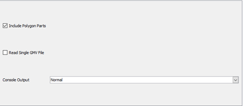
Reader GUI |
 |
|
Include Polygon Parts |
Include polygon parts will include parts with polyhedral and/or polygon elements. Default is off. |
|
Read Single GMV File |
Toggle this On to read only the file you have selected and only the timestep represented by this file will be available. If off, this will read all the GMV files as a transient dataset, when you select only one. Default is off. |
|
Console Output |
Normal - Minimal console output, only for errors. Verbose - Normal output plus information about the model. Debug - Full information for the developer to diagnose a problem. Use this output to help to diagnose a problem or to send it to Ansys. |
The following topics are included in this section:
The following topics are included in this section:
Reads a CFX results (.res) file. Currently reads version 16.1-0 and earlier.
Simple Interface Data Load
Load your geometry/results file (typically named with a suffix .res) using the Simple Interface method.
Advanced Interface Data Load
Load your geometry/results file (typically named with a suffix .res) using the Advanced Interface method to customize the read, for example to read transient geometry (see below).
|
Data Tab |
|
|
Format |
Use the CFX-5 format. |
|
Set file |
Select the geometry/results file (.res) and click this button |
|
Format Options Tab |
|
|
Set measured |
Select the measured file and click this button. |
|
Reader GUI |
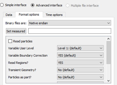 |
|
Variable User Level |
Allows you control of a number of variables read based on a call into the CFX API. The allowable choices are as follows: Level 0 - Read in all variables Level 1 - (default) Level 2 - Level 3 - |
|
Variable Boundary Correction |
Variable values are corrected using a boundary value correction if this toggle is Yes. YES - (default) Variable values adjusted using a boundary value correction. No - Variable values are not corrected. |
|
Read Regions? |
YES - Read regions. This is the default. No - Do not read regions. Note: For 2022 R2, we have changed the default for Read Regions to YES. This change was made to improve the ability for the Turbo surfaces initialization, allowing the needed part separation which is not always available with the boundary specification (Read Regions is set to No). If you experience a regression in part creation due to this change, you can change Read Regions back to No. You can set this preferences in the Format dialog for future use. |
|
Transient Geometry? |
A flag to the reader if the data is transient. Note: By default, a transient .res file will fail to load unless this is changed to Yes. CFX transient data will have a .res file and a series of .trn files (one for each timestep) located in a subdirectory. The res file will have the names of the .trn files, the time value and path. If the data is changing variables only then the .trn will not contain the mesh. If the mesh is moving, then you must turn on the Include Mesh in the Transient Result options so that the solver will write mesh information to each .trn file. Failure to do this results in a static, unmoving mesh over time. No - (default). Yes - Coordinates only. |
|
Particles as Part? |
If this is Yes, then EnSight reads in the particle data as a separate EnSight point part. No - (default) Do not read in particles as a separate EnSight Part. Yes - Read in the particles as a separate EnSight part |
Caveat
Elemental values of Overset variables will be available only on
Overset cell zones and boundaries attached to them.
Limitations
The CFX reader does not support Polyflow Classic data.
The CFX solver does export to EnSight Case Gold format.
CFX-Pre expressions that are saved during the simulation may show up in EnSight, otherwise expressions can be calculated within EnSight's calculator.
Variables that end in _beta have no units (for example,
*_beta).
EnSight contains limited turbomachinery capabilities that are available in Beta. To have more details on this, see Ansys EnSight Beta Features.
Transient Blade Row (TBR) CFX model data is not supported in EnSight.
EnSight does not support a CFX multi-configuration simulation; the resulting .mres is not a recognized EnSight reader file format and reading should not be attempted. However, you can directly read the .res file(s) in the simulation subdirectories.
See Read Data.
The following topics are included in this section:
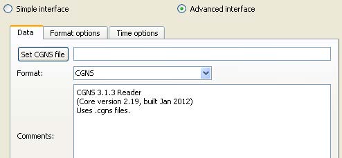
Legacy Reader
There are three CGNS readers in EnSight: this one, the CGNS-XML Reader, and a legacy, unsupported reader (CGNS-Legacy) which is unavailable by default, but can be made visible in the list of readers in the data section of the preferences.
Some information on this reader is available at:
$CEI/ensight251/src/readers/cgns/README.txt
Simple Interface Data Load
Load your geometry/results file (typically named with a suffix .cgns) using the Simple Interface method.
Advanced Interface Data Load
Load your geometry/results files (typically named with a suffix .cgns) using the Advanced Interface method.
|
Data Tab |
 |
|
|
Format |
Use the CGNS format. |
|
|
Set cgns |
Select the geometry/results file (typically .cgns) and click this button. For models contained in multiple files, wildcards or a special executive file can be used here. See Special Notes. |
|
|
Format options tab |
 |
|
|
Set measured |
Select the measured file and click this button. |
|
|
Include any Element sets defined. These are sets of full elements which are generally some logical subset of the total number of elements. Default is on. |
||
|
Include Face/Edge Set Parts |
Include any Face or Edge sets defined. These are some logical set of particular faces and/or edges of full elements. Default is on. |
|
|
Include NodeSet Parts |
Include any Node sets defined. These are generally the subset of nodes needed for the Element, Face, or Edge sets above. As such, they are generally not needed as separate parts, but can be created if desired. Default is off. |
|
|
Include local elem res comps (if any) |
Include the local stresses components, etc that are in the element's local system. A simple example is a bar (such as a truss element), which only has tension or compression in the element's axial orientation. Such an element would have an axial stress variable. Other elements would have appropriate result component variables. Default is on |
|
|
Include Tensor derived (VonMises, etc.) |
For tensor results, calculate scalars from the following derived results (principal stress/strains, and common failure theories): Mean Equal Direct VonMises Min Principal
Octahedral Mid Principal Intensity Max Principal Max Shear
By default, all 9 of these will be derived. You can control which are created by this toggle, with an environment variable. Namely, setenv ENSIGHT_VKI_DERIVED_FROM_TENSOR_FLAG n where n = 1
for Mean only 2 for VonMises only 4 for Octahedral only 8 for Intensity only 16 for
Max Shear only 32 for Equal Direct only 64 for Min Principal only 128 for Mid
Principal only 256 for Max Principal only 512 for all
or any legal combination. example: for VonMises and Max Shear only, use 18. Default is on. |
|
|
Regular Part Creation Convention |
Parts will be created according to the following: |
|
|
Use Part Id |
Part Id (this is the default) |
|
|
Use Property Id |
Property Id |
|
|
Use Material Id |
Material Id |
|
|
Element Vars as |
Single element values |
Element results (whether centroidal or element nodal) will be
presented as a single value per element. Therefore will be
|
|
Averaged to node values |
Element results (whether centroidal or element nodal) will be
averaged to the nodes without using geometry weighting. Therefore will be
|
|
|
Geom weighted average to node values |
Element results (whether centroidal or element nodal) will be
averaged to the nodes using geometry weighting. Therefore will be
|
|
|
Ave to node values <by parts> |
Element results (whether centroidal or element nodal) will be
averaged to the nodes without using geometry weighting. Therefore will be |
|
|
Geom weighted ave to node <by parts> |
Element results (whether centroidal or element nodal) will be
averaged to the nodes using geometry weighting. Therefore will be
|
|
|
Spatial Decomp Multiple File Search |
Normally, a single CGNS file is specified and read. Namely, the model is neither decomposed spatially into more than one file, not temporally into more than one file. Therefore the first option is the default. However, when a model is spatially decomposed, it can be read as long as it conforms to one of the other three options below. |
|
|
Use file specified |
Opens only the file you specify. This is the default. |
|
|
Numbered in same dir |
Opens and combines data from all filenames with the same pattern, but different ending numbers, that are in the same directory. file.cgns.1 <= specify this one file.cgns.2 ... file.cgns.9 |
|
|
Same name in numbered dirs |
Opens and combines data from all filenames with the same name, but in different numbered subdirectories. dir1/file.cgns <= specify this one dir2/file.cgns ... dir9/file.cgns |
|
|
Numbered in numbered dirs |
Opens and combines data from all filenames with the same pattern, but different ending numbers, that are in different numbered subdirectories. dir1/file.cgns.1 <= specify this one dir2/file.cgns.2 ... dir9/file.cgns.3 |
|
|
Doing Structured as: |
Structured |
will cause originally structured parts to be created as structured parts in EnSight. This is the default. |
|
Unstructured |
will cause originally structured parts to be created as unstructured parts in EnSight. |
|
|
Var naming convention |
Use Content Field (if provided) |
Variable names will be what is in the Content field, if provided. If not provided, they will be the VKI dataset name. This is the default. |
|
Use VKI dataset name |
Variable names will be the VKI variable dataset name (which are reasonably descriptive). |
|
|
If Sections, which: |
Which section will be used to create the variable |
|
|
First |
The first section will be used (this is the default) |
|
|
Last |
The last section will be used |
|
|
Section Num (below) |
The section number entered in the field below will be used |
|
|
Separate Vars per Section |
A separate variable will be created for each section. |
|
|
If Section Num, 1-based integer value: |
If the previous option is chosen to be Section Num, then the value in this field is the 1-based section number to use to create the variable. |
|
Special Notes
Special file input methods for temporally decomposed models. Namely, a file per timestep. Possible file input methods:
Normally, a single .cgns file would be specified. Therefore, for a non-decomposed model, or to view one particular time step, you would enter the desired file.
If multiple .cgns files exist because of transient results, you can use a wildcard (asterisk) in the name of the file, or subdirectory.
Example 2.2: For the Situation Where Multiple .cgns Files Reside in the Same Directory
/mydirectory/cfd_out.cgns.1
cfd_out.cgns.2
specify: /mydirectory/cfd_out.cgns.*
Example 2.3: For the Situation Where Multiple .cgns Files with the Same Name Reside in Their Own Subdirectories
/mydirectory/sub1a/cfd_out.cgns
/sub2a/cfd_out.cgns
specify: /mydirectory/sub*a/cfd_out.cgns
Example 2.4: For the Situation Where Multiple .cgns Files with Different Names Reside in Their Own Subdirectories
/mydirectory/sub1a/cfd_out.cgns.1
/sub2a/cfd_out.cgns.2
specify: /mydirectory/sub*a/cfd_out.cgns.*
Note: In general, you can't have a mixture of these two examples with this method. Namely, the following cannot be properly specified with this method:
/mydirectory/cfd_out.cgns.1
/sub2a/cfd_out.cgns.2
You would need to either copy the .cgns file in the subdirectory to the data directory, or you will need to create a subdirectory for each .cgns file in the data directory, and move the .cgns files into those subdirectories. You could obviously take advantage of symbolic links to avoid actually moving any data.
Your other alternative is to use method 3) below.
However, having said that, there is one special case where you can use this method with the final file not being in the pattern subdirectories.
Special case requirements:
All but the last file is in the pattern subdirectories.
Each of the files in the subdirectories must have the same name, and it must be the same as the one in the parent directory.
Example 2.5: Special Case
/mydirectory/sub1a/cfd_out.cgns
/sub2a/cfd_out.cgns
cfd_out.cgns
specify: /mydirectory/sub*a/cfd_out.cgns
and the
/mydirectory/sub1a/cfd_out.cgns,
/mydirectory/sub2a/cfd_out.out
files will be loaded.
Then the
/mydirectory/cfd_out.cgns
file will be loaded.
You can create a special executive file in which you list all of the .cgns files.
This would allow them to be placed in or anywhere below the data directory. Therefore, you could handle the mixture discussed in step 2 above.
Rules for this special file:
The file must be named exactly: MULTILPLE_CGNS
The .cgns files must be one per line in this file.
They must NOT have a full path, because the path to the MULTIPLE_CGNS file will be prepended to them.
There is no concept of comment lines, so no extraneous lines (even empty lines) are allowed.
Example 2.6: Example 1 Above, Specified in This Manner
/mydirectory/cfd_out.cgns.1
cfd_out.cgns.2
MULTIPLE_CGNS
where MULTIPLE_CGNS file would contain just 2 lines, like:
------------------ dashed lines are NOT in the file
cfd_out.cgns.1
cfd_out.cgns.2
------------------
Example 2.7: Example 2 Above, Specified in This Manner
/mydirectory/sub1a/cfd_out.cgns
/sub2a/cfd_out.cgns
MULTIPLE_CGNS
where MULTIPLE_CGNS file would contain just 2 lines, like:
------------ dashed lines are NOT in the file
sub1a/cfd_out.cgns
sub2a/cfd_out.cgns
-------------
Example 2.8: Example 3 Above, Specified in This Manner
/mydirectory/sub1a/cfd_out.cgns.1
/sub2a/cfd_out.cgns.2
MULTIPLE_CGNS
where MULTIPLE_CGNS file would contain just 2 lines, like:
------------- dashed lines are NOT in the file
sub1a/cfd_out.cgns.1
sub2a/cfd_out.cgns.2
-------------
And for the mixed mode situation:
/mydirectory/cfd_out.cgns.1
/sub2a/cfd_out.cgns.2
MULTIPLE_CGNS
where MULTIPLE_CGNS file would contain just 2 lines, like:
------------- dashed lines are NOT in the file
cfd_out.cgns.1
sub2a/cfd_out.cgns.2
-------------
Warning: If you have a CGNS file that reads fine into EnSight on Linux, but fails to read into EnSight on Windows, you may have encountered an infrequent issue in the CGNS API that can cause CGNS file to only be readable on specific platforms. Specifically, the issue may occur when a CGNS file is exported by an application written in Fortran on Linux. The file reads fine in EnSight under Linux but fails to read in EnSight under Windows for all CGNS readers. The issue is triggered by differences in Intel FPU configurations in the Linux Fortran vs the Windows C/C++ runtime environments. It can be difficult to predict when this can happen, but the probability tends to be higher in files with larger meshes. While we have seen the issue occasionally in Fortran/Linux data being read on Windows, we do not have any examples of a CGNS file written on Windows being unable to read under Linux.
The workaround is that CGNS includes a conversion/copy application with the installation under Linux. This tool makes a copy of the input file using the CGNS API. It is designed to upgrade the file to the latest version of the CGNS file format. It can also fix the issue related here because it reads and writes the file using the C/C++ runtime and its associated FPU configuration. You run this converter on Linux (where the file can be read). You can either install and run this on Windows using the WSL2 Linux subsystem or on another Linux system.
Instructions for Running the Converter Under Window WSL2
Install
cgns convert 3.4and run the following:sudo apt install cgns-convert cgnsconvert -h bad_file.cgns good_file_hdf5.cgns Output: converting ADF file bad_file.cgns to HDF5 file good_file_hdf5.cgns ADF input file size = 15182606336 bytes HDF5 output file size = 15164976960 bytes
Note: The example command line will also convert the file from ADF to HDF5 format. You should then be able to load good_file_hdf5.cgns into EnSight on Windows.
See Read Data.
Note: In 2025 R1, the CGNS-XML reader is now hidden by default.
Existing scripts will continue to work using this reader. If you specifically require this reader, you can turn its visibility back on in > .
We suggest using the CGNS reader instead, which is fully available and supported going forward. In a future release, we anticipate completely removing the CGNS-XML reader.
The following topics are included in this section:
Reads a Spymaster .spcth file.
See the following file for current information on this reader.
$CEI/ensight251/src/readers/cth/README.txt
Simple Interface Data Load
Load your geometry/results file(s) (typically named with a suffix .spcth) using the Simple Interface method.
Advanced Interface Data Load
Load your geometry/results files (typically named with a suffix .spcth) using the Advanced Interface method.
|
Data Tab |
|
|
Format |
Use the CTH format. |
|
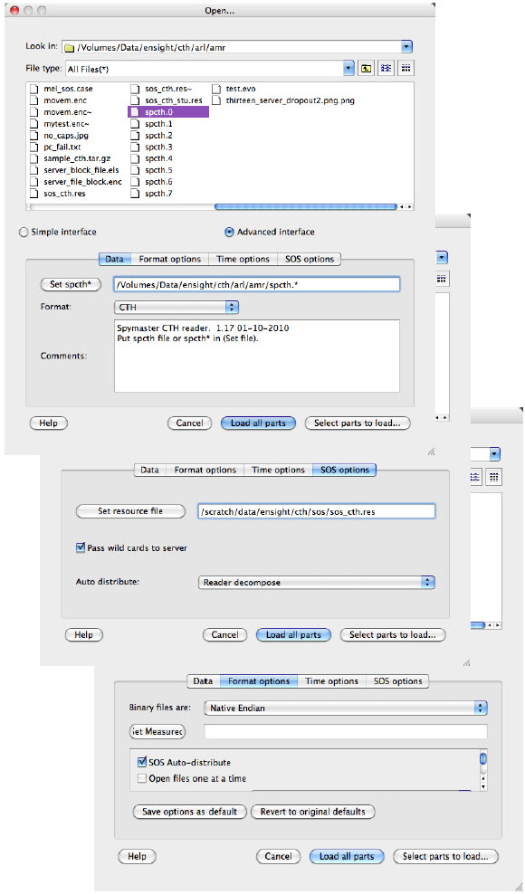
Set spcth* |
To read one Spymaster file, put the CTH Spymaster file (typically named something filename.spcth) into the (Set) Geometry field. To read in multiple, related CTH Spymaster files (for example several files solved in parallel) as follows: filename.spcth.0 filename.spcth.1 filename.spcth.2 Put an asterisk ' |
|
Format Options Tab |
|
|
|
Select the measured file and click this button. |
|
Reader GUI |
User controls as shown below are available:
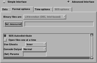 |
|
SOS Auto-distribute |
When running EnSight in SOS mode, turn this ON (default) to tell the reader that you want it to intelligently distribute the data among the servers. Turn it off if you have already distributed the spcth files into different directories, or on different machines and want to use a Case SOS file to assign the spcth file(s) to EnSight Server(s) manually. |
|
Open files one at a time |
When running EnSight in SOS mode, turn this ON to tell the reader that you want it to only open one of the spcth files at a time. When this is OFF (default) every server process may open a number of the files simultaneously. This could be a problem if you have a thousand files and a thousand servers and your process reaches a limit with too many files opened at once. |
|
Use Ghosts |
Ghosts are invisible elements between the Server geometries that allow for interpolation of data results rather than extrapolation. Ghosts can be inner (default) - use only the inner ghosts between blocks all - use both inner as well as ghosts around blocks none - no ghosts normal - read in ghosts as normal cells. outer zero - read in the inner and outer, but zero the variable values on the outer locations. This is useful to create end caps on the isosurfaces. |
|
Console Output |
Normal - Normal console output Verbose - Extra output useful to the user to understand their data better. Debug - Extra output often useful in debugging problems. |
|
(Set) Params |
Allows user to enter parameters to change the behavior of the reader, often for debugging purposes. For example to limit the number of blocks in the part to 102, enter the following:
|
Special Variables
EnSight's CTH reader has several special variables useful for
understanding SOS data. FILE_ID is the file ID number for each cell.
BLOCK_ID is the block index. And SERVER_ID is the
server that has the data.
SOS details
You can start up SOS using enshell, or the legacy Case SOS file, or the legacy resources file (.res) file, each discussed elsewhere in this manual.
Reader-distribute is the default behavior of EnSight. In Reader Distribute mode, if you have more files than servers, files are distributed to servers in a round-robin fashion according to file size to even the load. If you have more servers than files, servers are allocated to files according to total file size per server. In Reader Distribute mode, all files must be available to all servers.
Shown below are graphical user interface images showing sample user input for a sample SOS read of 8 spatially distributed spcth files into EnSight SOS using a resource .res file.
If you decide that you want to manually distribute the files, then you must move the sets of files into separate directories, create the SOS case file with different directories and the filename* casefile, and toggle the reader SOS auto-distribute OFF in the Format Options above.
See Problems for more tips problem-solving your SOS visualization.
See Read Data.
The following topics are included in this section:
The DVS reader reads in either in-situ data coming from a running solver or from a previouisly written cache. When running in-situ it can also optionally write the cache of data to be read in later.
This reader currently supports all EnSight element types for unstructured data. For structured data it accepts parallelepiped and curvilinear data.
It currently only supports scalar and vector variables (no complex or tensors yet).
When a cache is written the data will be split into multiple folders based on the number of EnSight servers it was written with. Each of these folders contains a sqlite database for metadata along with a hdf5 file containing the payloads of data received.
DVS Files
To be able to use the in-situ connection, a DVS file must be provided an example of contents are below:
#!DVS_CASE 1.0
SERVER_PORT_BASE=50055
SERVER_PORT_MULT=1
CACHE_URI=hdf5://localhost/D:/temp/testing_no_ensight
The initial #!DVS_CASE 1.0 should be provided to tell
us what version of the file you are using. Currently, 1.0 is recognized.
SERVER_PORT_BASE: This should be set to a starting
port for servers to listen for incoming data.
SERVER_PORT_MULT: This is used when running EnSight
in SoS mode with multiple servers. It is used to increase the port number for each server
sequentially. I.E. 1 means ports 50055, 50056 etc. 2 would be ports 50055, 50057, etc. 1
should be fine in most cases.
CACHE_URI: If this is not present, data will be in
memory only. If it exists with a location, a cache will be written to that location if
possible.
This is the format:
<cache_domain>://<machine>/<location>
| Section | Description |
| <cache_domain> | Only hdf5 is currently supported. |
| <machine> | localhost in most cases, not currently used, will be in future options. |
| <location> | Absolute or relative on disk location, for example, D:/temp/testing or /my/path/to/cache if an absolute location is not given it will be relative to the working directory EnSight was launched from. |
Limitations
Does not accept tensor or complex variable data.
Does not auto decompose data. If data was written with X servers it must be read in with X or less servers.
Simple Interface Data Load
Load your DVS file using the Simple Interface method.
Advanced Interface Data Load
Load your DVS file using the Advanced Interface method.
| Data Tab | |
| Format | Use the DVS format. |
| Set .dvs file | This field should point to a valid .dvs file which describes a cache location to open or in-situ parameters to stream in data. |
| Set cache URI | Can be used instead of the CACHE_URI section of the DVS file. |
| Format Options Tab | |
| Binary files are | Unused by reader |
| Set measured | Unused by reader |
| Verbosity level | Determines the verbosity of debug out by reader. Set to Full to get all debug information. |
| Time options Tab | |
| Monitor for new time steps |
Off: Reader expects a cache to be valid and read in. No in-situ connections. Jump to end/Stay at current: Will start an in-situ connection waiting for data. Will wait until the first timestep has been received before giving control back to EnSight. |
The following topics are included in this section:
Misc Notes
The Exodus reader links to the exodus routines in libexoIIc.a and the netcdf routines in libnetcdf.a. You must have these libraries to compile and run the ExodusII reader, and they are installed with EnSight.
Variable names that end in x,
y, z will be treated as components of a vector. For
example, the variables vel_x, vel_y,
vel_z will be treated as a vector named vel_vec.
Case is ignored in matching variable names.
GUI Control of Reader
Reader behavior can also be controlled in the Data Reader GUI via check boxes and fields. The environment variables, if set, are used to set the default values for the GUI.
Summary
Selecting the first file of any multi-file Exodus dataset will cause the reader to load the entire dataset. Selecting a non-first file of a spatially decomposed or a temporally decomposed dataset will cause the reader to load only that file. If you want to load only the first file, the Read Selected File Only toggle must be turned ON and that file selected. If a dataset is both spatially and temporally decomposed and a non-first file is selected, only the selected spatial decomposition will be loaded and it will be loaded for all time steps.
Single File - No Decomposition
If the file is not decomposed spatially nor temporally, then you will have only one Exodus file. Selecting this file will load all of the geometry and variables over all time. The file will be named something like file.e.
Spatially Decomposed Files
If the files are decomposed only spatially as shown below (each file contains a portion of the geometry over all time), then EnSight will behave as follows:
To load all the files automatically, choose the first file.
To load a particular file, choose that file. If only the first file is desired toggle ON the Read Selected File Only reader option.
file.e.4.0
file.e.4.1
file.e.4.2
file.e.4.3
Temporally Decomposed Files
If the files are decomposed only temporally as shown below (each file contains all the geometry but only for a subset of the total time), then EnSight will behave as follows:
To load all the files automatically, choose the first file.
To load a particular file, choose that file. If only the first file is desired toggle ON the Read Selected File Only reader option.
file.e
file.e-s0002
file.e-s0003
Spatially and Temporally Decomposed Files
If the files are decomposed spatially and temporally, as shown below, then there is a portion of the geometry in each file (indicated by 4.0, 4.1, 4.2, and 4.3) and a portion of the total time range in each file (indicated by s0002, and s0003) as shown below. EnSight will behave as follows:
To load all the files automatically, choose the first file.
To load only one portion of the geometry, choose any non-first file (for example: choosing file.e.4.1 will load the .1 geometry over all time steps, choosing file.e-s0002.4.0 will load the .0 geometry over all time steps).
To read only one file, choose the file and toggle ON the Read Selected File Only reader option.
file.e.4.0
file.e.4.1
file.e.4.2
file.e.4.3
file.e-s0002.4.0
file.e-s0002.4.1
file.e-s0002.4.2
file.e-s0002.4.3
file.e-s0003.4.0
file.e-s0003.4.1
file.e-s0003.4.2
file.e-s0003.4.3
Advanced Multiple File Naming
This reader supports two extensions to the filename fields. The first supports Exodus datasets where the geometry changes at some point in time. In this case, a new Exodus file (or set of files), is used for each set of solution times. To support this feature, insert wildcard characters (for example, * and ?) in the filename that expand to the name of the first files in each timeset.
The second extension allows for multiple files to be read as part of
the same timeset (for example, domain decomposed files). This feature takes the form of a tag
(<X:Y>) appended to the filename. The value of "X" is the number of files in the
timeset and "Y" is the sprintf () format string on the integer (%d)
formatting options) for expanding an integer argument into a string. http://en.wikipedia.org/wiki/Printf#printf_format_placeholders
For example, if a dataset consists of the following files:
Times 0-10 Times 11-15
| foo.e.03.00 | foo.e-s0002.03.00 |
| foo.e.03.01 | foo.e-s0002.03.01 |
| foo.e.03.02 | foo.e-s0002.03.02 |
Where the foo.e.* files contain timesteps 0
through 10 and the foo.e-s0002.* files contain timesteps 11 through
15. Also, each timeset is spatially decomposed into 3 subfiles, which each contain some
portion of the dataset for the given timesteps. For this dataset, use the file pattern
foo.*.03.<3:%0.2d> to tell EnSight there are multiple
timesets and to generate the filenames for each timeset by replacing the <..> substring with a number from 0 to 2 as generated using
sprintf() and %0.2d.
Note: The <...> marker must be the last part of the filename. The * will wildcard the timeset number and the <...> specifies the spatial decomposition.
More Info
See the following file for current information on this reader.
$CEI/ensight251/src/readers/exodusII/README.exodus
Simple Interface Data Load
Load your geometry/results file (typically named with suffix .e, .ex0, .ex, or .ex2) using the Simple Interface method.
Advanced Interface Data Load
Load your geometry/results file (typically named with suffix .e, .ex0, .ex, or .ex2) using the Advanced Interface method.
|
Data Tab |
|
|
Format |
Use the Exodus II format. |
|
Set exo |
Select the geometry/results file (typically .ex1 or .ex2, or .ex0) and click this button. If there are multiple Exodus files in the solution set, select the first file to load all of the data. |
|
Format Options Tab |
|
|
Set measured |
Select the measured file and click this button. |
|
Reader GUI |
When you choose Exodus reader, and toggle on the button, then click on the format options tab, you will see a number of options for controlling the reader behavior. Each of the choices in the data reader dialog has a corresponding Environment variable described below that you can set to control the default behavior. If you find yourself repeatedly toggling on or off choices in the Format options tab of the data reader dialog, consider setting specific Environment variables to change the default behavior of the reader.
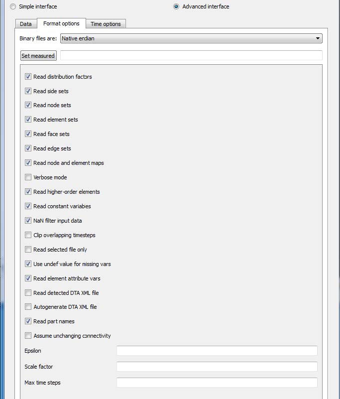 |
|
Read Distribution Factors |
Sets in Exodus can have distribution factor weights. If this is ON (default ON) then distribution factors will be read in as variables defined only on Set parts. The Environment variable ENSIGHT_EXODUS_DF can be used to set the default value (1 is ON, 0 is OFF). |
|
Read Side Sets |
Toggle ON (default) to read Side set parts. The Environment variable ENSIGHT_EXODUS_READ_SIDESETS can be used to set the default value (1 is ON, 0 is OFF). |
|
Read Node Sets |
Toggle ON (default) to read Node set parts. The Environment variable ENSIGHT_EXODUS_READ_NODESETS can be used to set the default value (1 is ON, 0 is OFF). |
|
Read Element Sets |
Toggle ON (default) to read Element set parts. The Environment variable ENSIGHT_EXODUS_READ_ELEMENTSETS can be used to set the default value (1 is ON, 0 is OFF). |
|
Read Face Sets |
Toggle ON (default) to read Face set parts. The Environment variable ENSIGHT_EXODUS_READ_FACESETS can be used to set the default value (1 is ON, 0 is OFF). |
|
Read Edge Sets |
Toggle ON (default) to read Edge set parts. The Environment variable ENSIGHT_EXODUS_READ_EDGESETS can be used to set the default value (1 is ON, 0 is OFF). |
|
Read node and element maps |
Toggle ON (default) to read node and element ids or labels (referred to in Exodus as node maps or element maps). There is no guarantee (particularly if using spatially decomposed Exodus files) that the node and element labels will be unique. If this option is toggled OFF then EnSight will ignore the labels in Exodus file and generate an internal numbering scheme guaranteed to have unique node and element ids. The Environment variable ENSIGHT_EXODUS_USE_NODEMAPS can be used to set the default value (1 is ON, 0 is OFF). |
|
Verbose Mode |
Toggle ON (default OFF) to output more detailed information to the server console. The Environment variable ENSIGHT_EXODUS_VERBOSE can be used to set the default value (1 is ON, 0 is OFF). |
|
Read higher order elements |
Toggle ON (default ON) to preserve higher order elements. Toggle OFF to down convert these elements to simpler elements (for example, convert a HEX20 into a HEX08). The Environment variable ENSIGHT_EXODUS_USE_HIGHERORDERELEMENTS can be used to set the default value (1 to preserve higher order elements and to 0 to convert these elements to simpler elements. |
|
Read constant variables |
Toggle ON (default ON) to load the variables that have a single value at each timestep (called Constants in EnSight). The Environment variable ENSIGHT_EXODUS_READ_CONSTANTS can be used to set the default value (1 to load constant variables and 0 to not load them). |
|
NAN filter input data |
Toggle ON to check all floats (geometry as well as variables) for IEEE nans and set to zero if nan (default ON). The Environment variable ENSIGHT_EXODUS_CHECK_NANS can be used to set the default value (1 to check all floats and 0 to not check floats). |
|
Clip Overlapping timesteps |
EnSight must have monotonically increasing time values in each successive timestep. Exodus files sometimes have overlapping timesteps. Toggle this ON, and when overlapping times are encountered, EnSight will truncate the former values and use the latter timesteps to construct the timeline. If this is toggled OFF (default) and EnSight encounters duplicate time values in subsequent timesteps it will apply the epsilon value (see Epsilon below) and increment the latter timestep so it remains monotonically increasing. With this option toggled OFF, EnSight will retain all timesteps but change the time values and is therefore not recommended. The Environment variable ENSIGHT_EXODUS_CLIP_TIMESTEP_OVERLAP can be used to set the default value (1 to truncate the timesteps with overlapping time ranges, and 0 to keep all timesteps). |
|
Epsilon |
A delta time value (default 1.0) to be substituted when a non-increasing delta time float value is encountered. If the reader detects two sequential time values that are not increasing the later solution time value will be set to the earlier time plus this epsilon value. This will have a cascading effect, shifting other solution times later as well. This is useful when the solution times are all the same value in the Exodus dataset. Set the Environment variable ENSIGHT_EPSILON to a positive float value to change the default value. |
|
Read Selected File Only |
Toggle ON to read one and only one file which is the selected file. Toggle OFF (default) to allow automatic pattern recognition (and loading) of certain categories of file naming schema as discussed in the beginning of this section. ENSIGHT_EXODUS_READ_SELECTED_FILE_ONLY can be used to set the default value (1 to read only one file and 0 to read all matching files in the schema). |
|
Use Undef value for missing variables |
Toggle ON (default) to return EnSight's undefined value when missing variable values are encountered (see EnSight Gold Undefined Variable Values Format ). Toggle OFF to return a value of 0.0 for missing variable values, which is the behavior of the reader prior to reader version 2.72). The Environment variable ENSIGHT_EXODUS_USE_UNDEF_VALUE can be used to set the default value (1 to return UNDEF and 0 to return 0.0 for missing variable values). |
|
Read element attribute vars |
Some elements have unique attributes (such as thickness for 2D shell elements). Toggle ON (default) to read in element attribute variables and OFF to not read these in. Use the Environment variable ENSIGHT_EXODUS_READ_ELEMENT_ATTRS to set the default value (1 to read these values 0 to not read them). |
|
Use detected DTA XML file |
Toggle this ON (default is OFF) to check for the existence of a .dta file (and read it in). The DTA file has extra metadata more fully describing the parts. Set the Environment variable ENSIGHT_EXODUS_USE_DTA_FILE to change the default (1 is read .dta file, and 0 is do not check). |
|
Auto generate DTA XML file |
Toggle this ON (default is OFF) to generate a stub .dta file from the Exodus datafile. Set the Environment variable ENSIGHT_EXODUS_AUTOGEN_DTA to change the default (1 generate stub .dta file, 0 is do not generate .dta file). |
|
Read part names |
Toggle this ON (default is ON) to read in the part names from the Exodus data file. Set the Environment variable ENSIGHT_EXODUS_USE_FULL_NAMES to change the default (1 to read in the part names from the Exodus data file, 0 to not read them in). |
|
Assume unchanging connectivity |
By default, with this Toggle OFF, when an Exodus dataset has multiple temporal files, the reader assumes that this is a changing connectivity file. Changing connectivity geometries lose some capabilities within EnSight, such as the ability to interpolate variable values between timesteps. If you know your temporally decomposed dataset does not change connectivity, then toggle this ON to tell EnSight to not make this a changing connectivity dataset; the dataset will become a changing coordinates geometry (which does allow interpolation between timesteps). To change the default, set the environment variable as follows: ENSIGHT_EXODUS_ASSUME_UNCHANGING_CONNECTIVITY to a value of 1 and the toggle will appear ON. |
|
Scale Factor |
Enter a positive float value (default 1.0) to be used as a scale factor for geometry and vectors (not for scalars). Set the Environment variable ENSIGHT_EXODUS_SCALE to a positive float value to change the default value. |
|
Max time steps |
By default, EnSight can read from an Exodus file while the simulation code is updating the Exodus file. For allocation purposes, EnSight needs an absolute maximum number of steps that will appear in the data file(s) during your EnSight session. Currently, the maximum number of time steps that EnSight will read is given here as 100000. Increase this value if your solver may exceed this amount. A value less than or equal to 1 will disable the ability to check for new time steps. Note: This field is ignored on Exodus files with HDF5 as the underlying format, as HDF5 files cannot safely be read and written simultaneously. Set the environment variable ENSIGHT_EXODUS_MAX_TIMESTEPS to change the default. For details on how to use this capability in EnSight, see How To Change Time Steps and the Advanced section in How To Load Transient Data). |
SOS
You can start up SOS using enshell, or the legacy Case SOS file, or the legacy resources file (.res) file, each discussed elsewhere in this manual.
There can be no more servers than the number of sub-files however (but fewer servers are legal and in most cases, recommended). Finally, if there are sub-files, the number and the naming convention must be the same over all timesets.
The Exodus reader does the decomposition automatically when running in Server of Server (SOS) mode, which is called Reader-distribute mode. In Reader Distribute mode, data is distributed to servers in a round-robin fashion. In Reader Distribute mode, all files must be available to all servers.
If you decide that you want to manually distribute the files, then you must move the sets of files into separate directories, create the SOS casefile with different directories and the filename* casefile, and toggle the reader SOS auto-distribute OFF in the Format options above.
Shown below are graphical user interface images showing sample user
input for a sample read of spatially distributed Exodus files (4 processors) into EnSight
SOS using a simple 4-server resource (sos.res) file as follows. Also
shown is the geometry colored by the Server number calculated using the
Calculator Function
ServerNumber (which is an excellent way of showing the allocation of
the geometry among the EnSight Servers. See the Problems section of the Use Server of Servers for more tips problem-solving your
SOS visualization.
#!CEIResourceFile 1.0
SOS:
host: localhost
SERVER:
host: localhost
host: localhost
host: localhost
host: localhost
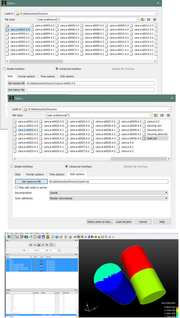
See Read Data.
The following topics are included in this section:
A FIDAP Neutral file contains all of the necessary geometry and result information for use with EnSight.
A neutral file is produced by a separate procedure defined in the FIDAP documentation. If the data is time dependent this information is also defined here.
Simple Interface Data Load
Load your geometry/results file (typically named with a suffix .fdneut) using the Simple Interface method.
Advanced Interface Data Load
Load your geometry/results file (typically named with a suffix .fdneut) using the Advanced Interface method.
| Data Tab | |
| Format |
Use the FIDAP Neutral format. |
| Set geometry |
Select the geometry/results file (typically .fdneut) and click this button |
| Format Options Tab | |
| Set measured |
Select the measured file and click this button. |
See Read Data.
The following topics are included in this section:
This EnSight reader uses the FLSGRF READER API LIBRARY from FlowScience in order to read data from a Flow3D flsgrf* output data file as well as the prpgrf* files written out in preprocessor mode (which contain only one timestep). FlowScience is no longer supporting compressed formats with the *.fgz and *.dat suffix.
Requirements
If any extra FlowScience API debug files are desired from the EnSight session, the FLSGRF API requires that the user have write permissions in the directory where the flsgrf file resides.
THE FLSGRF API is only available for Windows 32-bit, 64-bit, Linux 32-bit, and Linux 64-bit platforms.
EnSight attempts to implement the latest FLSGRF API and the FLSGRF API should read flsgrf files written by older versions of Flow3D.
Data Types
There are several kinds of data available in a Flow3D flsgrf output file, each with its own EnSight timeset: Restart, Selected, Fixed, and Particle data.
Restart Data
By default, there are 11 restart timesteps per solution: t=0 and an additional ten each spaced at 1/10th of the total simulation time. You can change this frequency in Flow3D using the plotting interval (PLTDT) in the PREPIN input file.
Selected Data
This consists of selected variables output at a higher number of timesteps. Restart and selected data can both be available in the data file.
Fixed Time Group
This data does not change over time. It consists of simulation parameters such as binary flags used to activate physical models as well as mesh data.
Parallel Solution
If multiple flsgrf files (flsgrf1.dat, flsgrf2.dat, ...flsgrfn.dat) from a parallel run and the number of servers equals the number of files, then choose the first one (flsgrf1.dat) and choose decomposition spatial and the remainder will be automatically loaded. Each server reads only one of the spatially decomposed files therefore dividing up the memory requirements. For temporal decomposition, load all the spatially decomposed files flsgrf*.dat and choose temporal decomposition. In this mode, each server loads a separate timestep therefore speeding up transient post-processing.
Particle Data
If particles are present in the simulation they will be present in the Restart data. If you request particle information in the Selected data (from their project file where anmtyp(i)='part') then particle information will also be available in the Selected data timesets.
Particle data is not imported into EnSight by default. To import this data, Choose the Multipart Flow3d reader then click on the Format options tab and select the type of Particle data that you wish to import.
Geometry is STATIC in EnSight unless Particle data is imported and then the geometry is CHANGING CONNECTIVITY because the number of particles can change with each timestep.
Technical Notes
All block part variable data is cell-based (per element data). All particle variable data is node-based (per node data). All FSI/TSE data is node-based (per node).
To visualize the fluid in the block try creating an isosurface of the
Fluid Fraction using an isosurface value of
0.51. Now to see the surrounding structure, make another
isosurface with a value of 0.51 using the
Cell_Volume_Fraction_Fixed variable. Click on the paint
can icon and change your shading to smooth to improve the isosurface look. To
see the fluid as an isovolume, File →
Command and type in test:
simple_isovolume_off then make an isovolume from
0.5001 to 1.0 using the Fluid
Fraction and again change its shading to smooth.
To see detailed information about variables, blocks, boundary conditions, etc., choose Console Output Debug as described below.
This reader makes use of Timesets. Each of the variable types has it's own Timeset timeline and EnSight merges them all together. For details on using these timesets see the advanced section of the Change Time Steps in the Ansys EnSight How-To Manual.
Ghost Cells
Ghost cells are invisible elements that help EnSight to interpolate variable values. For example, Ghost cells between blocks allow for a smooth transition of the isosurface of the fluid surface at part block boundaries. Ghosts that are not used have a zero value for the variable, and must be removed: removal of ghosts at a symmetry surface allows for smooth mirroring of the part(s).
Units
If the units are specified in a known unit system in the data file, then EnSight can convert them to any of the other known unit systems at read in. Also, EnSight can annotate by the units for any of the variables (those not non-dimensionalized).
Updated Info
$CEI/ensight251/src/readers/multi_flow3d/README.txt
Simple Interface Data Load
Load your Flow3D file (typically named flsgrf*) using the Simple Interface method.
Advanced Interface Data Load
Load your Flow3D file (typically named flsgrf*) using the Advanced Interface method.
|
Data Tab |
|
|
Format |
Use the Flow3d-Multiblock format. |
|
Set flsgrf |
This field should be an flsgrf or prpgrf file. If multiple flsgrf files (flsgrf1.dat, flsgrf2.dat, ... flsgrfn.dat) from a parallel run, then choose all using an asterisk (flsgrf*.dat) in place of the numbers, or one by specifying the particular file (flsgrf1.dat). |
|
Format Options Tab |
|
|
Format Options |
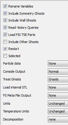 |
|
Rename Variables |
Variables are renamed by default to be easier to interpret for Flow3D users. |
|
Include Symmetry Ghosts |
Flow3D includes the following boundary conditions: symmetry, wall, continuative, periodic, specified pressure, specified velocity, grid overlay, outflow and interblock. Ghosts are always included in periodic, specified pressure, and inter-block boundary conditions. Ghosts are optional (using a toggle) for the following boundary conditions.
By default, symmetry ghosts are removed so that mirroring in EnSight has no seam. However toggling ON this flag will include the symmetry ghosts for example for inviscid flow using the symmetry condition to simulate a wall. |
|
Include Wall Ghosts |
Flow3D includes the following boundary conditions: symmetry, wall, continuative, periodic, specified pressure, specified velocity, grid overlay, outflow and interblock. Ghosts are always included in periodic, specified pressure, and inter-block boundary conditions. Ghosts are optional (using a toggle) for the following boundary conditions.
By default, wall ghosts are removed so that the EnSight fluid/wall interface does not show up using the isosurface of the fluid fraction. However toggling ON this flag will cause the fluid/wall interface to show up using the isosurface of the fluid fraction. |
|
Include Other Ghosts |
Flow3D includes the following boundary conditions: symmetry, wall, continuative, periodic, specified pressure, specified velocity, grid overlay, outflow and interblock. Ghosts are always included in periodic, specified pressure, and inter-block boundary conditions. Ghosts are optional (using a toggle) for the following boundary conditions.
By default, these other ghosts are removed so that the EnSight fluid/wall interface does not show up using the isosurface of the fluid fraction. However toggling ON this flag will cause the fluid/wall interface to show up using the isosurface of the fluid fraction. |
|
Read History Queries |
The flsgrf file often includes xy plotting data in the form of history data that is loaded into EnSight as pre-defined Queries accessible by clicking on the Query/Plot icon or below the part list in the Parts/queries tab. Default is ON. |
|
Load FSI TSE Parts |
Fluid-Structure Interaction and Thermal Stress Evolution unstructured parts (hexa8 and tet4's) and their associated stress, strain, temperature, displacement and blanking (STATUS) nodal variables are loaded into EnSight by default. A TSE (thermal stress evolution) component is a region in the fluid, where the fluid solidified and a structural analysis is performed in the solid in response to thermal gradients. An FSI (fluid-structure interaction) components, is a solid region in the fluid where the flow-induced structural deformations in turn, influence the flow, requiring simultaneous structural and fluid flow solution There can be only one TSE part in a simulation. |
|
Restart |
Load the variables on the Restart Timeline. Default ON. |
|
Selected |
Load the variables on the Selected Timeline. Default OFF. |
|
Particle Data |
By default, particle data is not read into EnSight. Choose the appropriate timeline to read in the Particle data. |
|
Console Output |
Use this flag to determine the amount of output to the console. Normal - Usually only echo errors to console. Verbose - Normal output plus an echo of every Fluent part that is in the dataset, whether it is interior or not, whether it is skipped, what variables are defined for which parts, and to echo it's EnSight Part number. Debug - Verbose output plus more detailed output and progress through the reader routines often valuable for understanding and reporting problems. Also detailed block information, variable information, boundary condition information, and timeset information |
|
Treat Ghosts |
Ghost elements are invisible elements that help EnSight to interpolate variable values. Ghosts can be read in as Ghost cells, as normal (visible) cells, or they can be not read in at all.
|
|
Load Internal STL |
The flsgrf file sometimes includes surface, boundary condition, or other important surface geometry on one or more timelines. Default is to load None, but the pulldown allows you to choose Selected, Restart, or Static STL geometry timelines. |
|
FS Meta File Output |
The FlowScience reader API, optionally writes out optional performance and debug files when a flsgrf file is opened if you have write permission. These can help to speed up reading the second time a file is opened or to understand the details of the read or to diagnose a failed read. However, if multiple users each with different file mask permissions attempt to open a flsgrf file on a shared network hard drive, the writing and overwriting of these files becomes problematic and can cause a read to fail. The safest option, if others may follow your read of a given file, is to choose to not write out these optional files. The API offers four options on opening a file named, for example, flsgrf: None - write out no additional files Performance - writes out c-flsgrf, flsgrdr, g_flsgrf, and t_flsgrf files. Debug - writes out the flsout.rdr file All - writes out both Performance and Debug files. |
|
Units |
Convert units to selected type. FlowScience reader API allows the conversion of a known system units (CGS, SI or English) to another known system (CGS, SI, or English). EnSight will not convert from an unknown or unspecified unit system. Unchanged (default) - use the system of units in the data file CGS - Uses grams, centimeters, and seconds. SI - Uses kilograms, meters, and seconds. English - Uses slugs, feet, and seconds. |
|
Temperature Units |
Temperature units are always known (C, K, F, or R) and can therefore always be converted to any other unit system. Celsius - Convert to Celsius Kelvin - Convert to Kelvin Fahrenheit - Convert to Fahrenheit Rankine - Convert to Rankine Unchanged (default) use the temperature units in the data file |
|
Decomposition |
If running in EnSight SoS mode, the type of decomposition to use. None - Spatial - Traditional SOS mode in which each server is assigned one of the spatially decomposed block files. Temporal - Temporal SOS in which the data is not spatially decomposed, but rather each of the available servers reads a different timestep to speed up transient post processing. |
|
Set measured |
Select the measured file and click this button. |
Parallel Post Processing (SOS)
The Flow3D solver can calculate its solution in parallel. This type of solution writes out the data as separate files (flsgrf1.dat, flsgrf2.dat, flsgrf3.dat, ....), each containing one structured block. EnSight can read each of these files onto a separate server. Server 1 will read in the unstructured data plus block 1, server 2 will read in block 2, server 3 will read in block 3, etc.
You can create an SOS casefile (.sos), which maps out which server loads what data and start EnSight up in SOS mode, and just load the sos casefile directly. Alternatively, you can create a .res file to set up the servers, start up EnSight in SOS mode, and load the data as flsgrf*.dat, and, in the data reader dialog, choose the .res file and choose to allow sos to use the *. For more details (including a sample resource file and sample SOS case file and how to use them, see Use Server of Servers and search for Flow3D.
See Read Data.
The following topics are included in this section:
You have three methods to bring the data from Fluent into EnSight :
Reading the .cas.h5/.dat.h5 natively in EnSight.
Export EnSight Case Gold format from within Fluent.
Export Common Fluids Format (CFF Post) from within Fluent.
Which one to choose:
In general and common use cases requiring generic post processing needs, pick your variables of interest and export Common Fluids Format (.cas.post/.dat.post). In EnSight, use the Ansys Post File reader to import the .cas.post/.dat.post files.
For large data, where parallel is needed for capacity, pick your variables and export EnSight Case Gold nodal.
If you want to have a look at the raw restart data, you can load cas.h5/dat.h5, but be aware that some of the dat.h5 variable values are raw values intended for Fluent restart.
The preferred method is reading Case Gold exported directly from Fluent (which also works in parallel for large solutions). But if using the Fluent reader then .cas and .cdat is the next best method because the variable values from the .cdat will be corrected in Fluent prior to export to .cdat and available on all parts and correctly exported from Fluent. While the .dat variable file is readable and usable by the Fluent reader, it contains variable data that is only useful within Fluent for restart purposes and may not be accurate on all parts.
See the following files for current information on the Fluent direct reader.
$CEI/ensight251/src/readers/fluent/README.txt
The comments that follow are for the current Fluent reader. The reader loads ASCII, binary single precision, or binary double precision. The files can be uncompressed or compressed using gzip.
Note: This reader is used to load Ansys Airpak/Ansys Icepak .fdat data files (see AIRPAK/ICEPAK Reader).
Simple Interface Data Load
Load your geometry file (typically named with a suffix .cas) using the Simple Interface method.
Advanced Interface Data Load
Load your geometry and result files (typically named with a suffix .cas and .dat) using the Advanced Interface method.
|
Data Tab |
|
|
Format |
To use this reader, select the Fluent format. |
|
Set cas |
Select the geometry file (typically .cas or .cas.gz) and click this button. For transient data, use a single asterisk to replace the number (*.cas or *.cas.gz). |
|
Set cdat, dat or fdat |
Select the results file (typically .cdat or .dat or .dat.gz), and click this button. For transient data, use a single asterisk to replace the number (*.dat or *.dat.gz). Note: .fdat files (see AIRPAK/ICEPAK Reader) are also usable in place of the .dat file. The .cdat file is the automatic selection, followed by a .dat. If a .cdat or .dat file is collocated with a .fdat file, you will have to manually select the .fdat file and then click the Set cdat, , or button to use a .dat file variant. |
|
Format Options Tab |
|
|
Set measured |
Select the measured file (typically a .mea suffix) and click this button. If you have fluent particle data you can translate it into EnSight's measured data format and import the particles as measured data. |
|
Other Options using the current Fluent reader |
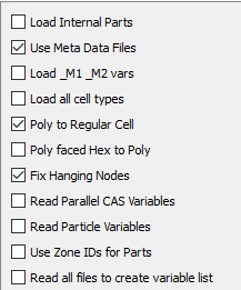 |
|
Load Internal Parts |
Toggle this ON to load the Fluent Internal Parts. This will show all the internal walls forming all the cell volumes. If you do toggle this on, then it is recommended that you click the button at the bottom of the data reader dialog, rather than , as you'll only want to load the interior parts of interest to save memory and time. Default is OFF. |
|
Use Meta Files |
Meta files are small summary files that contain highlights of the important locations inside each of the Fluent files. Allowing the EnSight reader to write out Meta Files that map the locations of important data can provide a significant speed up the next time you access that timestep. It is recommended that you leave this toggle ON. If you have write permission in the directory where your data is located, three types of binary Meta Files will be written when you first access each file, with extensions .efc for the .cas file, .efd for the .dat file and .efg for the time-history data. They are optional, and if you don't have write permission, the reader will take the extra time to read the entire .cas and .dat file to find the relevant data each time you come back to that timestep. |
|
Load _M1 _M2 vars |
Variables that end in |
|
Load all cell types |
Fluent cells have a boundary condition flag. By default (toggle OFF) EnSight loads only the cells with a boundary condition flag equal to 1 (one). Toggle this option ON to load all cells with a non-zero boundary condition. For example, if you have a part with cells of boundary condition 32 (inactive), EnSight will, by default not load this part. Toggle this option ON and EnSight will load this part. Note: Parts containing cells with a boundary condition of zero are never loaded. |
|
Poly to Regular Cell |
Fluent polyhedral cells when composed of the correct kind and number of regular faces can be converted to regular cells (tetrahedrons, hexahedrons, pyramids, or wedges) boosting EnSight speed and decreasing memory requirements. Toggle ON and reader checks each polyhedron to see if it can be converted to a regular cell (default) and OFF to not convert any polyhedral cells. There is very little slowdown during the read to do this and a big payoff for some datasets with large numbers of convertible polyhedra. Leave it on. |
|
Poly faced Hex to Poly |
Fluent hex cells that transition to a more refined hex mesh will sometimes have one or more of the quad4 faces subdivided into four quad4 faces. For example a hexahedral cell with one transition face will have the six full faces, and four subdivided faces for a total of 10 faces. Toggle ON and the subdivided faces are kept rather than the full face and the cell is changed into a polyhedral which will slow down EnSight performance, and greatly increase memory. The polyhedral also will have hanging nodes (see the next toggle). Toggle OFF (default) to convert the hex element to a six-sided hex which will be adjacent to four smaller cells rather than completely connected to them slowing down EnSight's adjacency searching. The default is thought to be the lesser of two evils. |
|
Fix Hanging Nodes |
Some Fluent polyhedral cells and all transition hex cells converted to polyhedrals will have hanging nodes. A hanging node is a node not shared by at least 3 faces. A polyhedral element with hanging nodes is not water tight and can cause real problems in EnSight, so it is best to leave this toggle ON (default) and only turn it OFF for experimental purposes. |
|
Read Parallel CAS Variables |
For parallel investigation, if the user toggles on read .cas variables, this option creates two new elemental scalars: ELEMENT_INDEX and PARTITION only if the data is solved in parallel and has partition section(s). This is primarily useful to visualize the Fluent geometric decomposition of parallel solutions. |
|
Read Particle Variables |
This will read particle coordinates and variable data from the .dat file. The number of particle parts is equal to the number of injections. |
|
Use Zone IDs for Parts |
A heterogeneous mix of serial and parallel solution files will result in a jumbled part ordering between CAS files. Toggle this ON to use the part zone id to reorder the parts consistently from .cas file to .cas file using the first file loaded as the canonical order. |
|
Read all files to create variable list |
Some transient datasets have different variables in the different .dat files. If this is OFF (default) then only the last .dat file will be used to create the variable list. If ON, then all .dat files will be used to create the master variable list. Regardless of the option, a variable will be assigned the EnSight Undefined value at time steps where it is undefined. |
|
Console Output |
Use this flag to determine the amount of output to the console. Normal - Usually only echo errors to console. Verbose - Normal output plus an echo of every Fluent part that is in the dataset, whether it is interior or not, whether it is skipped, what variables are defined for which parts, and to echo it's EnSight Part number. Debug - Verbose output plus more detailed output and progress through the reader routines often valuable for understanding and reporting problems. |
|
Time Values |
Use Filename Numbers will read the sequential numbers at the tail of the filenames and adjust them by making the first number 0 and shift all subsequent values. That is, file4000001.cas, file4000004 ... file4000020 is as follows: timestep 0 has time value 0.0, timestep 1 has time value 3.0, and timestep n has time value 19.0. Use Time Steps will make timestep and time value the same for example: timestep 0 will have time value 0.0 and timestep 5 have time value 5.0. Read Time Values (default) will open each file and find the exact time value using the 'flow-time' keyword. This means that every file has to be opened and searched. Failing that it defaults to the Calc Const Delta. Calc Const Delta reads a delta time from one file using 'physical-time-step' keyword, and calculates the time values by multiplying the delta value by the adjusted filename number. Failing that, it defaults to the Use Filename Numbers option. It is essential that your time values are correct for some calculations (for example, if you are going to do pathline tracing). Keep in mind that if your timesteps are uniform then you can use the 'Use Time Steps' option and just scale your time values using the Time Options tab in the data reader dialog. If your timesteps are not uniform, but your File Numbers are proportional to your timesteps then you can select Use Filename Numbers and then scale the time values using the Time options tab in the data reader dialog. |
Node and Elem IDs
Parts have node and element ids to enable querying your data. Node ids are created from the coordinate global node. Element ids are created as follows. Face part elements are uniquely numbered according to their zone index. Cell part elements are uniquely numbered using their zone index added to the total number of faces. So a dataset with 100 face elements and 300 cell elements would have the face elements number 1-100 and the cell elements numbered 101-400. In Verbose mode, the element id range for each part are written to the console.
.CDAT File
The variables in the Fluent .dat file are restart variable values that may require Fluent algorithmic manipulation in order to see values reflecting the actual flow physics. EnSight is not equipped with the physics found in Fluent, therefore reading the .cas and the .dat results in variable values missing (e. g. symmetry plane is missing variables) or wrong (velocity vectors are not parallel to the symmetry plane, or no-slip wall velocity is undefined rather than zero). The workaround, from within Fluent, is to export the variable values into the .cdat file (Fluent applies the physics to the .dat variables and then exports them to the .cdat file(s)) for all the part(s).
The EnSight Fluent reader has been updated to support Fluent 19.2 .cdat files. To take full advantage of this improved capability, the Fluent user will select the Fluid Part(s) within Fluent and export all variables of interest into the .cdat file. This will export properly extrapolated elemental variable values for all the fluid(s) as well as all the surfaces defined from the fluids. The user will then enter the .cas and the .cdat file into the geometry and results fields, respectively in the data reader dialog. The .cdat is the preferred form for reading variable values and should be used at all times over the .dat file(s).
Because the variables from the .cdat file are potentially different than those from the .dat file, Fluent renames these variables from the .cdat file using lowercase text. Further, .cdat variables are always scalars; the Fluent reader currently reassembles velocity and wall shear vectors only, but some other vectors may be missing, showing up only as three scalar components. Users with old command files can continue to read the .cas .dat files which may continue to work (some special datasets that go from serial solution to parallel solution may have the part IDs reordered and won’t run correctly). Using a command file created with the .cas and .dat files on a .cas and .cdat will not work (nor will older context files restore) due to these variable name changes.
In addition, the CDAT format can be used to export surface geometry (walls, isosurfaces, clip planes, inlet parts, etc), to greatly reduce the size of the output and keep it tractable for post-processing and their corresponding nodal variables. If either surfaces or fluids are exported then the nodal or elemental variables exported will match the corresponding geometry, respectively.
However, if both the fluid and the user surfaces are exported together, then elemental fluid variables (with their normal names) and nodal user surface variables (named with prefix us_*) will be exported. The elemental fluid variables will be undefined on the user surface parts and the nodal user surface variables will be undefined on the fluid parts. This can cause confusion when working in EnSight. For example, if the user tries to use a boundary layer calculator function using on a user surface part, you must tell the function to use the velocity that is defined on the fluid part in order to make this calculation.
Tip: Better yet, get Fluent to calculate the variables you intend to post-process and just write them out on your user surfaces directly.
Variable Location
Variables that are cell-centered remain where they are found in the .dat file, that is the reader does not interpolate the cell-centered variables to the nodes. Fluent can export variable data to EnSight's Case Gold format at either the nodes (default) or at the elements (same as .dat file). Unfortunately older versions of Fluent export variables averaged to the nodes leading to flow into and out of walls which causes particles to stop prematurely and skews mass flow calculations. Later versions of Fluent consider boundary conditions prior to averaging the data to the nodes, yielding a much more realistic representation of the physics.
Variables Undefined
Not all variables exist on all parts in the .dat file. If you select a part and color by a variable and get undefined, then load the data using Verbose mode and take a look at the console. Your variable is probably not defined for this part and EnSight does not have the boundary conditions nor the solver physics algorithms to extrapolate variable values to boundary parts. Create a clip on the location of an interior part on a volume part if you want to see a plane with the values from the volume.
Extra Variables
EnSight will try to calculate extra CFD variables given the existing
DAT variables for your convenience.
gzipped files
Files that are gzipped can be read by EnSight. However, with large numbers of parts this can result in a substantial slow down in the access of variable information in the .dat file because this involves non sequential access (seeking around various places in the file rather than sequentially moving through the file in order) which has been shown to result in dramatic slow downs. The workaround is to simply ungzip your files prior to reading them into EnSight.
CAS Constants
Extra CAS Single Value Variables - A number of single value variables are read from the .cas file(s). These will show up in the EnSight Calculator named as follows.
PRESSURE_ABS - operating pressure (absolute)
PRESSURE_ABS_INIT - initial operating pressure (absolute)
GAMMA_REF - reference gamma, ratio of specific heats
VISCOSITY_REF - reference viscosity
TEMPERATURE_REF - reference temperature
PRESSURE_REF - reference pressure
DENSITY_REF - reference density
SPEED_SOUND_FAR - far field speed of sound
PRESSURE_FAR - far field relative pressure
DENSITY_FAR - far field density
R_ref - Calculated reference gas constant = PRESSURE_ABS / (DENSITY_REF
* TEMPERATURE_REF)
V_def - Calculated default velocity magnitude from x, y and z-velocity
default values
M_def - Calculated from V_def / SPEED_SOUND_FAR
UDS, UDM Variables
UDM and UDS variables now read in as
UDM_0, UDM_1, UDM_2... and
UDS_0, UDS_1, .... Fluent differentiates between
UDS (User defined scalar) and UDM (user defined
memory) as follows.
A UDS is a scalar variable for which a transport
equation can be solved (for example, transport of a red color from an injection nozzle into the
volume; convective terms, diffusive terms,.) The single terms of this transport equation
are programmed via UDF (user defined functions) in C and are run time libraries.
A UDM is a node-based value which also is
calculated using a UDF (for example, viscosity against local temperature and density). For
UDMs transport equations are not solved. Therefore they require less memory compared to
UDS.
UDMs and UDSs are available for additional physics which are not available in Fluent (for example one can use a UDM for the calculation of dust concentration in filter elements.
Limitations
If species data is available only in Fluent PDF format, then the EnSight reader will not create the Mass and Mole fraction variables.
Polyhedral Elements
There are two methods to import polyhedral elements into EnSight. The first is to try using the direct reader. This has the advantage that the direct reader will attempt to convert polyhedral elements back to regular elements, saving memory and speeding up EnSight. The second is to export EnSight Case Gold .encas file from Fluent in parallel, decomposed format. Case Gold has the advantage of currently Server of Server in parallel, which can distribute the many tasks to multiple servers and speed up post processing (requiring an EnSight Enterprise license, formerly gold or hpc).
Periodic Elements
The reader now supports rotational symmetry to provide continuous boundaries.
Particles
The reader should attempt to read particles if they are present in the file(s).
Included with EnSight is a Fluent particle file translator to
translate the Fluent .part file into an EnSight measured
(.mea) data file. To get help with this translator, type
$CEI/ensight251/machines/platform/flupart -h where platform is your hardware/OS architecture (for example,
linux_2.6_64 or apple_10.5,
win32, etc.).
Source code and README for this translator are locate $CEI/ensight251/translators/fluent/Particles/
This measured data file is entered in the measured data field under the Format options tab of the data reader dialog.
See Read Data.
Variable Names
The names of the variables are created within the EnSight reader using simply the ID
of the variable found within the variable file (.dat) mapped to a
reasonable text name found within the reader. However some of the variables are
unknown or internal to Fluent and therefore not named. The practice of this reader is to
show all variables and therefore the variable internal name is used. For example, the
variable SV_ARTIFICIAL_WALL_FLAG is an internal Fluent variable, and
there is no text name. So this name is used.
The following topics are included in this section:
The Fluent HDF5 reader is supplied with EnSight to read Fluent .cas.h5 and .dat.h5 restart files written in Fluent 2019 R1 and onwards. .h5 extension indicates that they are HDF5 files. This reader uses Ansys CFF SDK (R20.2) to read all the information from .cas and .dat HDF5 files. This reader relies entirely on CFF SDK to provide necessary information to create parts and variable list. Using the R20.2 SDK, some older files (circa 19.3-19.5) may fail to read. For those seen so far, reading them into Fluent 2020 R2 and saving again resolves the issue.
Note: For some datasets saved from a version of Fluent prior to 2020 R1, EnSight’s Fluent HDF5 Restart reader fails to read the .cas.h5/.dat.h5 file. Resaving these datasets using a version of Fluent of version 2020 R1 or later resolves the issue, and can be read into EnSight.
Simple Interface Data
Load Fluent geometry file (typically named with a suffix .cas.h5)
Advanced Interface Data Load
Load Fluent geometry and result files (typically named with suffix .cas.h5 and .dat.h5) using Advanced Interface methods.
| Data Tab | |
| Format |
To use this reader, use Fluent_HDF5 format |
| Set .cas.h5 |
Select the geometry file (typically .cas.h5) and click this button. For transient dataset, use a single asterisk to replace the number (*.cas.h5) |
| Set .dat.h5 |
Select the result file (typically .dat.h5) and click this button. For transient dataset, use a single asterisk to replace the number (*.dat.h5) |
| Support to .msh.h5 file | Select the geometry file (typically .cas.h5) and click this button. For transient dataset, use a single asterisk to replace the number (*.cas.h5). Reader supports reading Fluent mesh files (.msh.h5), instead providing (.cas.h5) select only (.msh.h5) file and click on |
| Format Options Tab | |
| Fluent HDF5 reader options |
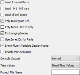 |
| Load Internal Parts |
Toggle this ON to load the Fluent Internal/Interior Parts. This will show all the internal walls forming all the cell volumes. If you do toggle this on, then you should click the Choose Parts button at the bottom of the data reader dialog, rather than Load all, as you'll only want to load the interior parts of interest to save memory and time. Default is OFF |
| Load _M1 _M2 vars |
Variables that end in _M1 and _M2 occur in Fluent unsteady flow. They represent the value of the variable at the prior iteration time and the time prior to that respectively. By default this toggle is OFF and these variables are not loaded. Toggle this ON to load these variables. |
| Load all cell types |
Fluent cells have a boundary condition flag. By default (toggle OFF) EnSight loads only the cells with a boundary condition flag equal to 1 (one). Toggle this option ON to load all cells with a non-zero boundary condition. For example, if you have a part with cells of boundary condition 32 (inactive), EnSight will, by default not load this part. Toggle this option ON and EnSight will load this part. Note: Parts containing cells with a boundary condition of zero are never loaded. |
| Poly to Regular Cell |
Fluent polyhedral cells when composed of the correct kind and number of regular faces can be converted to regular cells (tetrahedrons, hexahedrons, pyramids, or wedges) boosting EnSight speed and decreasing memory requirements. Toggle ON and reader checks each polyhedron to see if it can be converted to a regular cell (default) and OFF to not convert any polyhedral cells. There is very little slowdown during the read to do this and a big payoff for some datasets with large numbers of convertible polyhedra. Leave it on. |
| Poly faced Hex to Poly |
Fluent hex cells that transition to a more refined hex mesh will sometimes have one or more of the quad4 faces subdivided into four quad4 faces. For example, a hexahedral cell with one transition face will have the six full faces, and four subdivided faces for a total of 10 faces. Toggle ON and the subdivided faces are kept rather than the full face and the cell is changed into a polyhedral which will slow down EnSight performance, and greatly increase memory. The polyhedral also will have hanging nodes (see the next toggle). Toggle OFF (default) to convert the hex element to a six-sided hex which will be adjacent to four smaller cells rather than completely connected to them slowing down EnSight's adjacency searching. The default is thought to be the lesser of two evils. |
| Fix Hanging Nodes |
Some Fluent polyhedral cells and all transition hex cells converted to polyhedrals will have hanging nodes. A hanging node is a node not shared by at least 3 faces. A polyhedral element with hanging nodes is not watertight and can cause real problems in EnSight, so it is best to leave this toggle ON (default) and only turn it OFF for experimental purposes. |
| Use Zone IDs for Parts |
A heterogeneous mix of serial and parallel solution files will result in a jumbled part ordering between cas.h5 files. Toggle this ON to use the part zone id to reorder the parts consistently from .cas.h5 file to .cas.h5 file using the first file loaded as the canonical order. |
| Show Fluent Variable Display Name |
When this toggle is OFF legacy variable names are used, and when ON (default), the restart reader will match the Fluent variable ID from a variable map file ANSYS_FLUENT.xml (included in the EnSight install) which will allow EnSight to use the Fluent graphical user interface variable name. EnSight will use the variable map file to determine which variables to make available to the user. |
| Enable Part Grouping | This option allows the reader to group the Fluent cell zone and adjacent face zones. Default it is turned OFF. Unless both .cas.h5 and .dat.h5 are provided this option won’t work. |
| Console Output |
Use this flag to determine the amount of output to the console.
|
| Time Values |
Use Filename Numbers will read the sequential numbers at the tail of the filenames and adjust them by making the first number 0 and shift all subsequent values adhering to following situations.
|
| Project File Name |
Provide the name of the Fluent Project file (.flprj) written out by Fluent during the save of the .cas.h5/.dat.h5 (default empty). This project file, which is written by the solver, contains meta data regarding time value and .cas/.dat pairs. The specification of this filename, while optional, is encouraged when working with transient data to more robustly handle time values and .cas/.dat pairings. If no path is given (filename only), the routine will search the directory given by the .cas/.dat specification for this file. If no file is given, the reader will search the directory given in the .cas/.dat file specification. If a single file is found, the reader will attempt to use it. If multiple files are found (but none specified), the reader will not know which one to utilize and will therefore proceed with no project file. |
Node and Elem IDs
Parts have node and element ids to enable querying your data. Node ids are created from the coordinate global node. Element ids are created as follows. Face part elements are uniquely numbered according to their zone index. Cell part elements are uniquely numbered using their zone index added to the total number of faces. So a dataset with 100 face elements and 300 cell elements would have the face elements number 1-100 and the cell elements numbered 101-400. In Verbose mode, the element id range for each part are written to the console.
Part Order and Name
Part name and its order (sequence) appearing in EnSight’s part list is provided by CFF SDK. While reading transient dataset, the reader tries to maintain a global part list i.e. it scans all cas.h5 files and try to find out if number of parts are changing over time and creates a single part list which remains present at all the time-steps.
Note: EnSight needs all parts to be present in all the time-steps hence this scanning is required. This may increase initial read time while reading transient dataset. In a future release, the reader is expected to store/retrieve such a metadata upfront from CFF SDK to save considerable initial load time.
If you know that the number of parts does not change over time, and the number elements and nodes and connectivity does not change over time (for example, the geometry is static) you can avoid entering in the asterisk (for example, file*.cas.h5) for the geometry and only enter in one geometry file (for example, file0001.cas.h5) and EnSight will not scan all of the geometry files at first load, and EnSight will only load the geometry file once, therefore saving initial load time, and time required to change timestep.
Variable Location and Name
Fluent dat.h5 restart file has cell-centered solver specific variables’ data and this reader does not interpolate the cell-centered variables to the nodes. The reader attempts to identify the Fluent display variable name based on each variable’s sub section id provided by CFF SDK. If it’s not found reader may skip such variables with appropriate warnings.
Variables Undefined
Not all variables exists on all parts in .dat.h5 file. If you select a part and color by a variable and it is undefined; it means that selected variable is not defined for selected part and EnSight does not have the boundary conditions nor the solver physics algorithms to extrapolate variable values to boundary parts. Create a clip on the location of an interior part on a volume part if you want to see a plane with values from the volume.
Extra Variables
EnSight will try to calculate extra CFD variables given existing dat.h5 variables for your convenience.
CAS.H5 Constants
Extra single Value Variables - A number of single value variables are read from the .cas.h5 file(s). These will show up in the EnSight Calculator named as follows.
PRESSURE_ABS - operating pressure (absolute)
PRESSURE_ABS_INIT - initial operating pressure (absolute)
GAMMA_REF - reference gamma, ratio of specific heats
VISCOSITY_REF - reference viscosity
TEMPERATURE_REF - reference temperature
PRESSURE_REF - reference pressure
DENSITY_REF - reference density
SPEED_SOUND_FAR - far field speed of sound
PRESSURE_FAR - far field relative pressure
DENSITY_FAR - far field density
R_ref - Calculated reference gas constant = (PRESSURE_ABS /
(DENSITY_REF * TEMPERATURE_REF)
V_def - Calculated default velocity magnitude from x, y and z-
velocity default values M_def - Calculated from V_def / SPEED_SOUND_FAR
Polyhedral Elements
This reader will attempt to convert polyhedral elements back to regular elements, saving memory and speeding up EnSight.
Particles
Currently, the Fluent HDF5 reader handles Discrete Particle data and variables for those particles which are explicitly saved into the .cas.h5 and/or .dat.h5 files. The reader does NOT read in particles stored in other files (PDF files), nor particle information which is generated within Fluent Post interactively. For models which are running steady state continuous domain, you can have either steady particles, or unsteady particles computation. Only those situations where the particle data is explicitly written to the .dat.h5 or .cas.h5 files can be read by this Fluent HDF5 reader. It may appear like you see discrete particles in Fluent, but if they have not been explicitly written to the .dat.h5 or .cas.h5 file, the Fluent HDF5 reader will not be able to read them/provide them to EnSight. For models which are running transient continuous domain, the Fluent HDF5 reader will only be reading particle data from the .dat.h5 file, which may be coarser (temporally) than typically desired. We will attempt to address this shortcoming in the future Ansys Fluids Post format.
Variable Naming
The variables show in the variable list are determined by an internal, Ansys API. Therefore, the variables shown in this reader may differ from those shown in the Fluent cas/dat reader (which reads and shows all the variables directly from the .dat file). Further the variable names are also determined by the Ansys API and therefore may be different from the Fluent cas/dat reader, which names variables to traditional, reasonable, legacy text names.
Limitations
Part order is likely to be different than the legacy Fluent CAS/DAT reader
Overset grid variables are not yet available to correctly filter elements.
It does not read datasets older than 2019 R1.
It does not handle User Surfaces.
It does not handle nodal variables
Reading and handling additional variables are not supported by CFF SDK
Write permission is required for the directory containing .cas.h5/.dat.h5 files. The CFF API requires write access to the directory containing the .cas.h5/.dat.h5 files. You must ensure that write permission is available.
Note: The following table should be referenced to correctly understand the naming and display of the Yplus and Ystar values from Fluent HDF5 Restart into EnSight.
| Fluent Variable ID | Fluent Variable Name | EnSight Variable Name |
|---|---|---|
| SV_WALL_YPLUS | Wall_Ystar | YPLUS |
| SV_WALL_YPLUS_UTAU | Wall_Yplus | YPLUS_UTAU |
The following topics are included in this section:
The Forte reader is supplied with EnSight to read .ftind index file that is output from the Ansys Forte solver. Select the .ftind file to use the EnSight Forte to read your geometry and variable solution data into EnSight.
Note: If there are some geometry and variable data solution data present, then the reader will also read in xy query data into EnSight from the solver CSV output data.
The following topics are included in this section:
The LS-DYNA reader reads in a single or multiple unstructured C-binary d3plot files.
It supports bars, quads, bricks and thick shell elements.
Key File for Part Naming
Can use of Key file to name parts as follows:
Works only if Material IDs are in the d3plot file
Put key file name into Params field
Looks for *PART keyword in keyfile
$ in first column is a comment in keyfile
First non-comment line after *PART is used as partname if alpha or digit
Second non-comment line after *PART, 3rd integer is Material ID
If Mat'l ID in d3plot matches Mat'l ID in keyfile partname from key file is substituted for Material ID in EnSight name.
FEMZIP
The reader uses the publicly-available femunzip utility to unzip the compressed files. This unzip utility can be downloaded for free. The user must set the environmental variable FEMUNZIP_UTILITY_PATH to point to the location of this executable. The reader will call this executable on the d3plot file(s) to ensure that the file(s) are unzipped into a temporary folder prior to reading. A mapfile.txt pointing to the unzipped files will be created which will be used in subsequent runs avoid the need to unzip again.
CFD Data
The reader skips legacy CFDDATA sections, and reads instead the ICFD data from the incompressible CFD and incompressible CFD surface solvers.
DEM/DES
The reader now includes this particle data.
AMR
The reader can read AMR data even if the expected, first d3plotaa is not available.
Duplicate Timesteps
The reader skips duplicate timesteps, caused perhaps by double precision to float conversion.
Limitations
The reader has the following limitations:
Does not read airbag particle data
Doesn't support PACKED data (3 integers per word)
Skips over Rigid Road Surface Data.
Coordinate System: Global vs. Local: Beam stresses and strains are always output in the local r,s,t system. Per LSTC manual, stresses and strains of the other elements are generally in the global system. However, shells & thick shells have an option to output in local system (see LS-DYNA 960 keyword users manual page 9.18. flag CMPFLG). The reader has no way of knowing whether stresses and strains are output in the global or local system and just shows the values contained in the files.
See the following file for current information on this reader.
After the notation regarding
$CEI_HOME/ensight251/src/readers/ls-dyna3d204/README.txt,
users utilizing ALE Solutions will see additional variables listed as
el8_var01, el8_var02, etc. These variables
correspond to material volume fractions for the various of materials specified in the ALE
solution.
In addition, pressure is stored in the stress field variables and can be displayed by
computing a new variable in EnSight's calculator equivalent to the negative of the
average of the three normal stresses: 
Simple Interface Data Load
Load your d3plot file using the Simple Interface method.
Advanced Interface Data Load
Load your d3plot file using the Advanced Interface method.
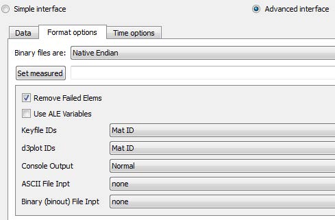
See Read Data
The LSTC-LS-DYNA Reader is a completely new, optimized implementation that uses an API written by LSTC (the authors of LS-DYNA) to read in a single, or a series of C-binary, d3* files (built on the d3plot framework), exported from the LS-DYNA solutions for post processing. Since the reader is built upon an API designed by the authors of the solver it should be expected to read the most current format updates (included FEMZIPPED data), and the broadest support for the families of solutions within the LS-DYNA application. The new reader is faster and provides a better LS-DYNA user experience than the legacy LS-DYNA Reader reader (which is still available, but not the preferred reader option).
Requirements
This reader uses version 0.1.41 of the LSTC API, which is included with your EnSight installation on Windows and Linux (Apple is not supported by the API). This supports d3* post processing files exported from version R12, and earlier versions of the LS-DYNA solver.
User Information
User messages from this reader (informational, warnings and errors) appear in the Message Box Overview. If problems are encountered, the user can choose Console Output in the Format Options tab in the Data Reader dialog with the LSTC reader chosen and the advanced toggle on. This will put a voluminous amount of debug output in the message box which can be saved and sent to Ansys support.
Supported Solution Types
Regular – Traditional, non-linear, explicit structural analysis using spherical particle hydrodynamic (SPH) point elements as well as bar, shell, solid, and thick shell non-linear element types.
Multi-Solver (MS) data is supported. This includes variables located on the Multi-Solver parts as well as Multi-Solver variables located on the structures. Variables undefined on individual nodes will assign the EnSight undefined value on those nodes, and will color those values using the undefined palette color (this is different from LS-PREPOST which assigns the undefined variables as 0.0).
Arbitrary Lagrangian Eulerian (ALE) – A moving Lagrangian mesh with Eulerian material flowing through it, that is used to model large deformation, fluid or fluid-like materials or fluid (eulerian) and structure (lagrangian) interaction. To visualize ALE fluids, try using isosurface or isovolumes using a material volume fraction variable.
Corpuscular Particle Method (CPM) data, used in airbag solutions, is now supported. Datasets with CPM data will result in a single CPM point part as well as CPM scalar variables.
Blast Force – This is a variant of a d3plot file, (commonly named blstfor* or *blstfor) that contains blast interface geometry and a number of elemental scalar blast variables (pressure, blast status flag, density, temperature, and velocity). The descriptions of these variables are found in the latest LS-DYNA® Database Binary Output Files document.
Interface Force – This is a variant of a d3plot file (commonly named *intfor or intfor*) that contains interface geometry and a number of interface elemental, scalar variables (forces, contact gap, surface energy, pressures, surface wear, and wear sliding distance). The descriptions of these variables are found in the latest LS-DYNA® Database Binary Output Files document.
Smooth Particle Galerkin (SPG) a high deformation particle formulation is supported which includes Implicit SPG (ISPG), and Element-free Galerkin (EFG) methods.
Noise Vibration & Harshness (NVH), Acoustics, Structural Dynamics, Modal, Random Vibration, Mechanical Shock, etc. This includes (but is not limited to) the following analysis families.
- ACC - Ansys Acoustic method solver file d3acc
- ACP - Ansys Composite PrePost solver file d3acp
- ACS - Car Cabin Acousics (ACS) solver file d3acs
- ATV - Acoustic Transfer Vector solver file d3atv
- EIGV - Eigenvalue/vector modal analysis file d3eigv
- ERP - Equivalent Radiated Power solver file d3erp
- FTG - Fatigue solver file d3ftg
- DRLF - Dynamic Relaxation Phase file d3drlf
- PSD - Power Spectral Density file d3psd
- RMS - Root Mean Squared file d3rms
- SSD - Steady-State Dynamics file d3ssd
Units
Neither LS-DYNA nor the exported post processing files support units. It is entirely the responsibility of the analyst to choose self-consistent inputs prior to running the analysis.
BINOUT XY Query Data
LS-DYNA saves xy queries in a standardized binary format in branches; each branch represents a category of xy data that was formerly an individual ascii file. Within a branch, a query might be a variable value over time, at a given location (nodal or elemental), within a set of grouped queries. A branch with a number of sets, a number of variables and a large number of node or element ids, can contain a very large number of XY query permutations. Also, these xy queries can have high sample rate time history data, resulting in a very large number of xy pairs.
Unfortunately, EnSight’s initial design of the query interface had in mind a relatively small number of queries with a relatively low sample rate. So, EnSight is currently very inefficient at the initial load of large number of queries especially those with a high sample rate. Currently EnSight reads in all of the xy data at the initial load and sends the xy pairs all up to the client, and has no mechanism to ‘activate’ queries, thus greatly increasing the initial load overhead), and then, after the load has no mechanism to organize and present and manage large numbers of queries (it lacks the ability to group and subgroup and tag queries in the query interface). So the limited implementation of binout data are currently considered for demonstration purposes only.
Currently the reader has limited support for two branches within the binary, binout datafile: spcforc, and nodfor time history data. When the binout file is entered into the second field in the data reader dialog, then the Message window will contain output indicating what branches are available and which ones are loaded. When nodal query data is available and supported, Query Parts (point parts) are created to spatially show nodal query locations in the graphics area and to allow users to right click on a query location node, and choose to plot the available queries at the selected location. However, given the current EnSight query interface limitations, the number of node or element ids is currently limited to 100 in order to keep the number of queries manageable. Support for time history branches will be added over time in this reader and the handling of large query data branches is expected to improve within EnSight as well in subsequent versions.
XY Query groups available in the BINOUT file
1. 'glstat'
Warn WARNING: Found 'glstat' xy data, but not implemented yet
2. 'matsum'
Warn WARNING: Found 'matsum' xy data, but not implemented yet
3. 'rcforc'
Warn WARNING: Found 'rcforc' xy data, but not implemented yet
4. 'spcforc'
number of XY Queries = 603
Parts and Materials
The reader supports the regular element types: spherical particles (as 0D point elements), bars (as 1D line elements), quads (as 2D surface quadrilaterals), bricks and thick shells (each as 8 node hexahedrals). Parts are formed out of element using material ids. Currently the actual material associated with the material id is unavailable in the post processing files and the LSTC API does not read the LS-DYNA input analysis key file (*.k or *.key) file where this information is found. Regular parts will be of KIND Regular. Part names will include the material ID as well as the part name, if it is available. For legacy datasets, where the part name is unavailable then only the material ID will be used as the regular part name.
Parts containing only points will also be formed for some branches of binout data to indicate the query location. These binout parts will be located in a Part group named XY_Query_Location, and each Query Part will named according to one of the branches: nodfor and spcforc and will have a point field, with each point representing a query location, and each point node id representing the query node id. A Query Part KIND is XY query locationnid. Initial query part visibility will be off, and the points will be represented initially as a cross and colored purple when the part is made visible to show the query locations. See Advanced for how to use the Query Parts.
When MS data is loaded, Parts that are Regular will be put within the Structural group (named using their material id and their part name, and they will have KIND Regular). MS parts will be grouped by their MS domain. Each MS part will be of KIND MS_Shell, MS_Solid, or MS_Beam to indicate their origin and their element type.
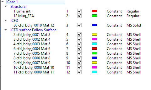
Transient
For transient data, Parts are either changing coordinates only (connectivity and nodes stay the same through time and only the xyz values of the nodal coordinates update through time) or changing connectivity (Nodes, xyz location, as well as the elements’ connectivity all change through time; this is called an adaptive mesh in LS-DYNA). This is an EnSight global, so if any part is changing connectivity, then all are changing connectivity.
If the data is a frequency analysis, then timesteps and time values become modes and frequency values. A case constant variable named Frequency is available as the actual frequency value.
Note: Since EnSight must have monotonically increasing time values, if either the time values or the frequency values are not monotonically increasing, then the timestep (0, 1, 2, …) is used as the time value. Use the variable Frequency to determine the actual frequency at a given timestep.
Variables
This reader creates single-value constants (transient single value per timestep), per part constant (transient single value per part), scalars, vectors, and plug-in (Python calculated) variables.
Variables are presented in the way that is most useful within EnSight (for example, Tensor variables are presented as Scalar components of the Tensor, such as Stress_XX) and named in a way that is most useful within EnSight (for example, noun_adjective_adverb): Strain_Effective_Plastic. Where variables are named within the Solution family (such as Multi-Solver, MS solution data) the variable name in the file is used (sans the forbidden characters Variable Creation). Variable values can be written in the database for certain parts in certain domains or for certain element types and not for others; the reader will handle this by defining the values where they are available and telling EnSight that the variable is undefined where it is unavailable.
Some variables are needed by you but are unavailable in the post processing files. They are made available as EnSight Python Plug in variables and include the following: Stress_Principal_Min, Stress_Principal_Min, Stress_Principal_Min, Stress_Tresca, Stress_Von_Mises, which will show up if the required six stress component scalars are available (Stress_XX, Stress_YY, etc. ). If these are activated, then the required six stress component scalars will also be activated, and an EnSight Python plug in will perform the required calculation to create these variables.
Multi-solver variables are available on MS part nodes or elements. Some
Electro-Magnetic variables may not have the correct name (appearing as
Var_01, Var_02, etc.) but their values appear
correct relative to LS-PREPOST.
The Centroid variable is currently undefined on
multi-solver elements. A workaround would be to use
the calculator function and
select from the Predefined
function parameters.
A single value is available for each scalar or vector component on each element. However that element may contain a number of values at each of the element integration points (IPs). You have the option at the time of the data read to choose one integration point location for the shell elements (inner, mid, or outer), or to combine them (min, max, or average of the three locations), or to combine all of them (if there are more than three, min, max or average of all the integration points. For the other elements, the user has the option of of min, max or average of all the integration points. The default for all element types is to present the max of all the integration point as the single value at that element. There is no option to change this choice except to reload the data and pick another option.
Caution: Variable names do not reflect your choice so it is possible to have two different sessions of EnSight with two different load options showing the geometry colored by the same variable name with very different values for the same dataset with no way of knowing except the command language, which variable load option was chosen at load time.
dir0/file_0_0.vtu
dir0/file_0_1.vtu
dir0/file_0_2.vtu
dir0/file_0_3.vtu
Displacement Variable – For regular analyses, this variable is created if the data is transient, and is not adaptive (not changing connectivity). This variable is created in the reader as the original coordinate vector subtracted from the current coordinate vector. If the data is modal then this variable is not created. The geometry in a modal analysis is shown undisplaced and in order to see the mode shape, the geometry must be deformed using the displacement icon, Display Displacements.
Delete Flag Variable – Filtering of failed elements is automatically turned on by the reader so that the EnSight server uses the Delete Flag value in order to filter out the visibility of the failed elements and doesn’t use them in calculations. For example, the total volume of a part comprised of solid elements will reduce over time as the Delete Flag indicates elements are failed and must be removed over time, Filter Part Elements.
Frequency Variables – For NVH analyses, some of the regular variables may be unavailable, and in there place there can be special frequency variables available. These are supported and are named using the _frequency_ embedded within the variable name, because they are very different, solution-specific variables.
LS-DYNA conditional variables are supported (a single variable location within the d3plot that is used to store values for completely different variables depending on the analysis type). This includes History variables. Which variable will remain unknown to the reader, because naming them requires the ability to parse the input (*.k, *.key) file, to figure out the analysis type and to use a lookup table to find the name. These variables appear in EnSight, for example, with cryptic names, such as Shell_Var01, Shell_Var02, etc where these particular variables can represent the following, depending on the analysis and/or material type, which should be known to the user.
Shell_Var01 - Lower plastic strain or Hourglass Energy
Shell_Var02 - Upper plastic strain, timestep, mass or added mass
OR
Solid_Hvar01
Solid_Hvar02
Apparent Variable Discontinuities Across Part Boundaries With ALE Solutions
LSPrePost interpolates variables globally (across parts), while EnSight interpolates
variables part by part. In the ALE solutions of LS-Dyna, the elemental-stored values can
have discontinuities from element to element, which can result in variable coloration
which illustrate this discontinuity between parts in the data. If this rendering
discontinuity is undesirable, there is method to handling discontinuities across parts by
issuing the command test: across averaging on in EnSight’s
Command dialog. Once turned on, you can then create a new variable
by using the ElemToNode() calculator function to interpolate the elemental
variable to the nodes (using averaging across parts) to generate a smoother nodal variable
field.
Simple Interface Data Load
Load your LS-DYNA file (typically named d3plot or file.d3plot, or any variation such as d3acc, etc.) using the Simple Interface (Simple Interface) method.
Advanced Interface Data Load
Load your LS-DYNA file (d3plot or file.d3plot, or any variation such as d3acc, etc.) using the Advanced Interface method.
|
Data Tab |
|
|
Format |
Use the LSTC-LS-DYNA format. |
|
d3file |
Choose one of the following that have been tested: d3plot, d3acs, d3acp, d3atv, d3eigv, d3erp, d3ftg, d3psd, d3rms, d3ssd, d3thdt, d3zcf, drlf , or choose other similar d3* or d* post processing file and click on the button. |
|
Binout |
Choose a binout file and click on the button. |
Format Options Tab 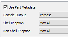 |
|
|
Use Part Metadata |
(default ON). Sets part KIND, MATERIAL (when this becomes available from the input (key) file, grouping, default coloration, point display type (if point part). This will create Query Parts if the binout file is selected in the second field and it contains a supported nodal query branch. This will also auto generate regular part groups, using the first three digits of the part id, if the part ids are greater than 100,000 and the if number of parts is greater than 200. |
|
Console Output |
Normal, Verbose, or Debug, default is currently Verbose. Errors and warnings are always printed out. Normal is typically minimal informational output, Verbose is output considered of interest to the curious user, and Debug output is designed as a window into the data itself, particularly useful for detailed, reporting of problems to Ansys support. |
|
Shell IP option |
, , or – A single IP of one of these three. , , or of the above three. , , or of all (if there are more than three). Default is . |
|
Non-Shell IP option |
, , or of all. Default is . |
Advanced
LS-Dyna sometimes writes out non monotonically increasing time values. EnSight does not support this type of data. The reader will attempt to tweak duplicate time values with a small delta time, and if that is not successful, then will make timesteps integers, starting at 0.0 and incremented by 1.0. Or, frequencies, which appear as separate timesteps will sometimes not be increasing with timestep. In this case, the reader will make a constant variable named Frequency, and will make the timesteps integers starting at 0.0 and incremented by 1.0.
The reader will send a flag up to EnSight for deleted elements, Filter Part Elements, Filter Parts.
Note: If all the elements are deleted on the timestep initially loaded, then the graphics parameters (zoom, look at, look from will be set wrongly) and you’ll need to do a fit when you change timesteps in order to update the graphics parameters.
If you have loaded binout data and you have xy query parts loaded, you can use these points to pick the location where you would like to see a query plotted. Make the query part visible that represents the binout branch of interest in order to see the points in the graphics area, then turn on node ids, and right click on the point of interest (see below, and notice the top of the right click menu says Part 3 nodfor, confirming that you’ve right clicked on a point in a query point part, in this example, node id 11501), then choose and see the pop up window so choose from all the queries that are available for node id 11501 as shown below. Click to see a plot of the selected queries in a single plot.
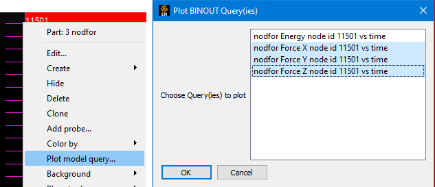
Limitations
The following are currently unsupported:
FEMZIP data
Rigid surface data
Key file metadata is unavailable
Material metadata linking the d3plot ID to the material name and properties is completely missing. Using the material properties
Units – Currently unavailable.
Workbench
The following topics are included in this section:
Reads any of the following (in preferred order):
The .dat file (which refers to .arc files in the directory)
or
One of the .arc files (which will get all .arc files of the same pattern)
or
The modified case file (for specific control).
See the following file for current information on this reader.
$CEI/ensight251/src/readers/dytran/README.txt
Simple Interface Data Load
Load your dytran file (typically named with a suffix .dat or .arc) using the Simple Interface method.
Advanced Interface Data Load
Load your dytran file (typically named with a suffix .dat or .arc) using the Advanced Interface method.
|
Data Tab |
|
|
Format |
Use the MSC/Dytran format. |
|
Set dytran |
The preferred input is the file with .dat suffix. The root name of this file will be used to find all .arc files in the directory which match the Dytran naming convention. And all parts of the model will be made available to EnSight. Additionally, this method allows for the most efficient setting for changing geometry, because it can glean some pertinent information thereto within the .dat file. Alternatively, you can enter one of the .arc files, and all .arc files in the directory which match the pattern will be found and used. Note: No widcards are needed - just select one of the .arc filenames. The third method is to enter a custom case file. This user generated ASCII file allows one to specify particular parts, etc. Since one can accomplish the same thing by only loading specific parts within EnSight, this method is probably obsolete. |
|
Format Options Tab |
|
|
Set measured |
Select the measured file and click this button. |
|
Format Options |
The following options are customized for the reader, in version 2.05 or later.
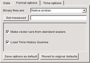 |
|
Make vector vars from standard scalars - Toggle on to have vector variables automatically generated from known standard scalar components. On is the default. Example: If toggled on, a vector variable named
|
|
|
Load Time History Queries - Toggle on to have all xy time-history queries (contained in pattern matching .THS files in the directory) loaded automatically into EnSight. On is the default. Note: These have traditionally been read into EnSight in the Query/Plot feature, but reading each .ths file as an external file. While this option still exists, it is not needed if this toggle is on. |
|
If you choose to not have the Dytran XY time-history data (from the .ths files) loaded automatically, or if you are using a prior version of the reader, you can later click on the XY Query/Plot icon and choose to load data from an external file in the pulldown, and choose the desired .ths file(s). For details, see Queries From External Sources.
See Read Data.
The following topics are included in this section:
Reads a t16 or t19 file (which is the preferred method).
See the following file for current information on this reader.
Simple Interface Data Load
Load your marc file (typically named with a suffix .t16 or .t19) using the Simple Interface method.
Advanced Interface Data Load
Load your marc file (typically named with a suffix .t16 or .t19) using the Advanced Interface method.
|
Data Tab |
|
|
Format |
Use the MSC.Marc format. |
|
Set t16/t19 |
This field should have the .t16 or .t19 suffix file. |
|
Format Options Tab |
|
|
Format Options |
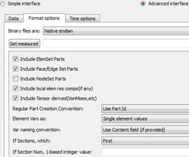 |
|
Include ElemSet Parts |
Include any Element sets defined. These are sets of full elements which are generally some logical subset of the total number of elements. Default is on. |
|
Include Face/Edge Set Parts |
Include any Face or Edge sets defined. These are some logical set of particular faces and/or edges of full elements. Default is on. |
|
Include NodeSet Parts |
Include any Node sets defined. These are generally the subset of nodes needed for the Element, Face, or Edge sets above. As such, they are generally not needed as separate parts, but can be created if desired. Default is off. |
|
Include local elem res comps (if any) |
Include the local stresses components, etc that are in the element's local system. A simple example is a bar (such as a truss element), which only has tension or compression in the element's axial orientation. Such an element would have an axial stress variable. Other elements would have appropriate result component variables. Default is on |
|
Include Tensor derived (VonMises, etc.) |
For tensor results, calculate scalars from the following derived results (principal stress/strains, and common failure theories): Mean Equal Direct VonMises Min Principal Octahedral Mid Principal
Intensity Max Principal Max Shear
By default, all 9 of these will be derived. You can control which are created by this toggle, with an environment variable. Namely, setenv ENSIGHT_VKI_DERIVED_FROM_TENSOR_FLAG n where n = 1 for Mean only 2
for VonMises only 4 for Octahedral only 8 for Intensity only 16 for Max Shear only
32 for Equal Direct only 64 for Min Principal only 128 for Mid Principal only 256
for Max Principal only 512 for all
or any legal combination. example: for VonMises and Max Shear only, use 18. Default is on. |
|
Regular Part Creation Convention |
Parts will be created according to the following: |
|
Element Vars as |
Single element values |
Element results (whether centroidal or element nodal) will be
presented as a single value per element. Therefore will be
|
|
Averaged to node values |
Element results (whether centroidal or element nodal) will be
averaged to the nodes without using geometry weighting. Therefore will be
|
|
|
Geom weighted average to node values |
Element results (whether centroidal or element nodal) will be
averaged to the nodes using geometry weighting. Therefore will be
|
|
|
Ave to node values <by parts> |
Element results (whether centroidal or element nodal) will be
averaged to the nodes without using geometry weighting. Therefore will be
|
|
|
Geom weighted ave to node <by parts> |
Element results (whether centroidal or element nodal) will be
averaged to the nodes using geometry weighting. Therefore will be
|
|
|
Var naming convention |
Use Content Field (if provided) |
Variable names will be what is in the Content field, if provided. If not provided, they will be the VKI dataset name. This is the default. |
|
Use VKI dataset name |
Variable names will be the VKI variable dataset name (which are reasonably descriptive). |
|
|
If Sections, which: |
Which section will be used to create the variable |
|
|
First |
The first section will be used (this is the default) |
|
|
Last |
The last section will be used |
|
|
Section Num (below) |
The section number entered in the field below will be used |
|
|
Separate Vars per Section |
A separate variable will be created for each section. |
|
|
Section Num |
If the previous option is chosen to be Section Num, then the value in this field is the 1-based section number to use to create the variable. |
|
See Read Data
The following topics are included in this section:
There are two Nastran readers: Nastran OP2, and Nastran OP2 (beta). Both read .op2 files, and the beta version additionally reads XDB files. This section documents only the Nastran OP2. It reads .op2 suffix files including most PDA Patran (PARAM POST = -1) and SDRC I-DEAS (PARAM POST = -2) files.
Limitations
Binary format only. (If you need to read ASCII, convert using the Nastran utility that will do this.)
Some non-linear and composite element types have not yet been implemented.
Recent Enhancements
Extra GUI options were added to allow the user control over part creation and variable extraction.
Location and displacement coordinate systems are now recognized and applied.
Multiple op2 files can be read by the reader, and therefore will appear in the same EnSight case. This is controlled by a simple ASCII file (.mop file).
The format of the .mop file is:
----------------------------------line 1: The word mop, in quotesline 2: The number of filesline 3 and up: Each op2 filename, in quotesNote: The .mop file extension has been added to the Nastran reader section of the ensight_reader_extension.map file (in site_preferences).
Rigid Body euler parameters are being read and passed to EnSight. (EnSight has also been modified to apply these rigid body parameters to the geometry and vector variables.) The specification of the rigid body file and the registration of which parameters apply to what - is also done in the .mop format.
The format of the .mop file, with rigid body information as well, is:
----------------------------------------------------------------------------
line 1: The word mop, in quotes
line 2: The number of files
line 3 and up: Each op2 filename, the euler parameter filename, the title of the rigid body transformation in the euler parameter file that apply to this .op2 file, and a unit conversion scale factor (if needed). All on one line per file, and all in quotes.
Example 2.11: .MOP File with Rigid Body Information
----------mop3"boom.op2" "rigid.eet" "BOOM" "1000.0""bucket.op2" "rigid.eet" "BUCKET" "1000.0""hframe_side.op2" "motion.eet" "HFRAME" "1000.0"Note: Since an euler parameter file contains the transformation information for many different "parts", the same file will generally be indicated for each .op2 file. However, this can be a different file for each .op2 file.
Also, the last column is not required - but is provided in the case that unit conversion is needed between the .op2 system and the euler parameter system. In our example, the .op2 system was in millimeters, while the translations values in the euler parameter file were given in meters.
Note: If there is an additional offset to the CG that is needed (other than that specified in the euler parameter file), these offsets can also be placed in the .mop file. Simply add three more columns containing the x, y, z offsets, like the following:
Example 2.12: Adding Offsets to the .MOP File
----------mop3"boom.op2" "rigid.eet" "BOOM" "1000.0" "883.7" "207.4" "0.0""bucket.op2" "rigid.eet" "BUCKET" "1000.0" "-10.5" "67.2" "7.89""hframe_side.op2" "rigid.eet" "HFRAME" "1000.0" "367.5" "-12.45" "0.0"You can also add a rotation order and yaw, pitch, and roll values on each of the file lines if the coordinate system must be re-oriented. These additional columns follow the same format as those in the EnSight Rigid Body (.erb) file.
The reader deals with timelines and needed interpolations between them. Generally, EnSight readers need only provide data at the given timesteps of a model. EnSight takes care of getting both ends of a time span and interpolating between them if needed. However, if rigid body motion is provided, the controlling timeline will be the rigid body timeline. Therefore, for a given rigid body timestep, we may fall between timesteps for the nastran model. This reader can interpolate properly for this situation.
Also, if not using rigid body, but are using multiple files - with different timelines - a combined timeline will be created and sent to EnSight. This also can require interpolation within the different files - and this is handled as well.
How variables are handled has been completely redone. The old reader simply presented the values of whatever was in the file. This lead to many different variables, depending especially on which element types were used. It also did not assure that some of the standard variables were available.
This reader now presents a standard list of the component and principal stresses/strains, and the useful failure theories. These values are obtained either by reading them from the file (if provided), or computing them from the data that is provided. We believe it is much more friendly and useful.
Because of the way that element variable values now may lead to nodal variables - requiring averaging, and because the way data is stored in a .op2 file is not always conducive to being used efficiently by EnSight - various caching schemes have been implemented to attempt to improve the efficiency of the reader. Hopefully appropriate trade-offs between memory and speed have been utilized. As such, it should be pointed out that one can color all parts by a variable about as quickly as coloring only one.
Static models with multiple loadcases use the Solution Time dialog to switch between loadcases. Therefore, a change of timestep in EnSight will actually change between loadcases.
Note: The preference within EnSight to have the Color Palette update at each time step is especially nice to have set for this situation.
.
README
See the following file for current information on this reader.
$CEI/ensight251/src/readers/nastran/README.txt
Simple Interface Data Load
Load your geometry/results file (typically named with a suffix .op2) using the Simple Interface method.
Advanced Interface Data Load
Load your geometry/results file (typically named with a suffix .op2) using the Advanced Interface method.
|
Data Tab |
|
|
Format |
Use the Nastran OP2 format. |
|
Set op2 |
Enter the .op2 filename if reading a single NASTRAN .op2 file, or a .mop filename if reading multiple .op2 files. The .mop file is an ASCII file listing .op2 filenames. See the description above or the README file indicated above for more details. |
|
Format Options Tab |
|
|
Set measured |
Select the measured file and click this button. |
|
Extra GUI |
The following parameters are available. They are described below.
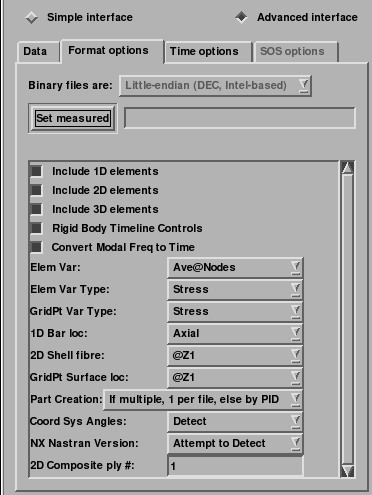 |
Format Options Parameters
The toggles and fields below are customized for the Nastran OP2 reader. They allow the user to specify basic options before the data is read. They may not all apply to any given model.
Include 1D Elements
Toggle on to include any 1D (bar, rod, etc.) elements.
Include 2D Elements
Toggle on to include any 2D (tri, quad, etc.) elements.
Include 3D Elements
Toggle on to include any 3D (tet, hex, etc.) elements.
Rigid Body Timeline Controls
Toggle on to have the geometry timeline controlled by the rigid body times (if present). If off, the flex body times in the .op2 file will control.
Convert Modal Freq to Time
Toggle on to compute solution time from the frequency field in the
file for eigen analysis (default is on). The is done with  . Toggle off to no perform this computation and instead read the
frequency value as the time.
. Toggle off to no perform this computation and instead read the
frequency value as the time.
Elem Var
This pulldown provides control over the way Nastran element values will be presented as variables within EnSight.
|
Centroidal |
produces |
|
Ave@Nodes |
produces |
|
Max@Nodes |
produces |
|
Min@Nodes |
produces |
Elem Var Type
This pulldown provides the choice of extracting either Strain or Stress from Nastran element values.
GridPt Var Type
This pulldown provides the choice of extracting either Strain or Stress from Nastran Grid Point values.
1D Bar Loc
This pulldown provides the choice of where along the bar (EndA, EndB) or across the cross-section (Pts 1-4), and what type of stress or strain to extract from Nastran bar elements.
| Axial | |
| Bend, EndA, Pt1 |
Combined, EndA, Pt1 |
| Bend, EndA, Pt2 |
Combined, EndA, Pt2 |
| Bend, EndA, Pt3 |
Combined, EndA, Pt3 |
| Bend, EndA, Pt4 |
Combined, EndA, Pt4 |
| Bend, EndB, Pt1 |
Combined, EndB, Pt1 |
| Bend, EndB, Pt2 |
Combined, EndB, Pt2 |
| Bend, EndB, Pt3 |
Combined, EndB, Pt3 |
| Bend, EndB, Pt4 |
Combined, EndB, Pt4 |
2D Shell Fibre
This pulldown provides the choice of which cross-sectional fibre (@Z1 or @Z2) to extract from Nastran 2D Shell elements.
GridPt Surface Loc
This pulldown provides the choice of which cross-sectional fibre (@Z1, @Z2, or @MID) to extract from Nastran 2D Grid Point surfaces.
Part Creation
This pulldown provides part creation choices (which are most useful when a .mop file is used to bring in multiple OP2 files together:
|
One Per File |
One part for each file will be created. If a single OP2 file is being read, all elements will be placed in a single part. If multiple OP2 files are being read, one part per file will be produced. |
|
By Property id |
Parts will be created by property id. According to how property ids were used in the OP2 file, this will generally create several parts per file. |
NX Nastran Version:
This pulldown provides you with some control over the changes that occurred in the element record length at NX Nastran version 4.0. This is needed because there is not a good way to determine the version used from the .op2 file itself.
|
Attempt to Detect |
Attempts to divine the version number, but may not always work correctly. If it can't tell, will default to less than version 4. |
|
Declare as >= 4.0 |
Declares the version to be 4.0 or greater, so doesn't go through the detection process. |
2D Composite ply:
This field allows the user to specify from which ply number to extract values from Nastran 2D composite elements
See Read Data.
The following topics are included in this section:
File → Open...
The File Selection dialog is used to specify which file you wish to read.
File → Open...
Handles steady state geometry with either steady state or transient variables. Steady state variables with multiple iterations will use each iteration as an EnSight timestep.
Not yet supported :
Ongoing solution. The reader cannot handle newly available timesteps or iterations (for example from an ongoing OpenFOAM solution) after the model has been read into EnSight the first time. Should new iteration or timesteps become available after the model was originally read into EnSight, the user must reload the dataset.
Command Line Data Load
To automatically start EnSight and load the current directory's
OpenFOAM dataset from the command line, type
ensight -Eensfoam. This will trigger EnSight to start up, look
for the current directory's system/controlDict file, and
automatically load the dataset into EnSight (using the default reader settings). This
reduces the number of steps to load the file into EnSight and therefore the real time
required to load the data, and provides a level of integration with this data
format.
Sample Data
A sample OpenFOAM dataset is included as a sample session with your install. To access the welcome screen, at the top menu choose Window → Welcome To... and load the Dam Break example session. Or, to load the same dataset manually, find the controlDict file in $CEI/ensight/other_data/openfoam.
Simple Interface Data Load
Load your OpenFOAM
controlDict file using the Simple Interface method. Or from the command line,
simply run ensfoam.
Advanced Interface Data Load
Load your OpenFOAM file using the Advanced Interface method.
|
Data Tab |
|
|
Format |
Use the OpenFOAM format. |
|
Set file |
This field contains the controlDict file. Clicking this button inserts the file name shown into the field. |
|
Format Options Tab |
|
|
Set measured |
Select the measured file and click this button. |
|
Other Options |
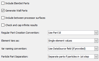 |
|
Include ElemSet Parts |
Include any Element sets defined. These are sets of full elements which are generally some logical subset of the total number of elements. Default is on. |
|
Generate Wall Parts |
Generate 2D Face Sets. Default is on. |
|
Include between processor surfaces |
If toggled ON and the data is from a parallel solution, then the surfaces between the processors will be generated as parts. Default is off. |
|
Check and cap infinite results |
If toggled ON and there exists values in the file that are beyond the 32-bit size limit (therefore creating 'inf' infinite values), they will be capped at a value just below that limit value. Default is off |
|
Regular Part Creation Convention |
Parts will be created according to the following: Use Part Id - Part Id (this is the default) Use Property Id - Property Id Use Material Id - Material Id |
|
Var naming convention |
Use DataSource field - By default variables are named using the variable filename. For example, "U" is velocity, "p" is pressure, etc. Use Content Field (if provided) - Known variables are given full, meaningful names, for example, "Velocity" or "Pressure". Use VKI dataset name - Long, hybrid variable name including the VKI variable dataset name. |
|
Particle Part Separation |
Parts will be separated according to the following: None - Remains within the original part Separate parts if particles in 1st step - Creates separate parts without particles (default) Separate for ALL parts (can be empty) - Creates separate parts for ALL original parts (even when empty) |
|
Element Vars as |
Single element values - Element results (whether centroidal or
element nodal) will be presented as a single value per element. Therefore will be
Averaged to node values - Element results (whether centroidal
or element nodal) will be averaged to the nodes without using geometry weighting.
Therefore will be Geom weighted average to node values - Element results (whether
centroidal or element nodal) will be averaged to the nodes using geometry weighting.
Therefore will be Ave to node values <by parts> - Element results (whether
centroidal or element nodal) will be averaged to the nodes without using geometry
weighting. Therefore will be Geom weighted ave to node <by parts> - Element results
(whether centroidal or element nodal) will be averaged to the nodes using geometry
weighting. Therefore will be |
See Read Data.
Simple Interface Data Load
Load your geometry file using the Simple Interface method.
Advanced Interface Data Load
Load your geometry and result files using the Advanced Interface method.
|
Data Tab |
|
|
Format |
Use the OVERFLOW format. |
|
Set geometry |
Select the grid file (grid.in or single x. file, e.g x.14200, see details below) and click this button. This file is a structured GRID file with FAST enhancements. |
|
Set results |
Select the results file and click this button. The results file is either a modified EnSight Results file (q.res) or standard plot3d Q-file (q.save or single q. file, for example, q.14200). The standard plot3d Q-file is a variable file for a single timestep and is optional. The modified EnSight results file directs the reader to handle multiple grid (x.) files and/or multiple variable (q.) files from transient simulations. If using a .res file, then enter only the first x. file into the set geometry field, and the .res into the set results field. Note: The Q-file(s) (and result file) may be located in a different directory than the grid file. |
|
Format Options Tab |
|
|
Set bounds |
The optional boundary file defines boundary portions within and/or across structured blocks. Note: This can be EnSight's boundary file format or a .fvbnd file. |
|
Set measured |
Select the measured file and click this button. |
Limitation
In order to automatically recognize the data as Overflow, the files must have the format x. and q. format (For example x.14000, x.14200, q.14000, and q.14200 would be appropriate filenames).
Note: The overflow reader can read in transient geometry files but these files must have the same number of zones (EnSight parts) at each timestep. Each zone can change in size (changing connectivity), but the total number of zones must remain constant throughout time.
Example .res file
For example, if you have files x.14400 to x.16000 and q.14400 to q.16000, then an example q.res file would be as follows. Then, put x.14400 into the set geometry and q.res into set results field and you will have transient geometry and variables.
2 1 1
10
1.0 2.0 3.0 4.0 5.0 6.0 7.0 8.0 9.0 10.0
14400 200
x.*****
q.***** S 1 Density q.***** S 5 Energy
q.***** S 2 3 4 Momentum
OVERFLOW Q FIle Variables
The variables of the flow information read by the OVERFLOW reader basically conforms to those read by the PLOT3D reader, and includes additional flow constants as well as additional Q variables such as Γ and possible turbulence field and species densities variables.
The Constant Variables include (where the first 4 are the standard PLOT3D constants):
|
|
= |
freestream Mach number Minf |
|
|
= |
angle-of-attack α |
|
|
= |
Reynolds number Re |
|
|
= |
iteration (file) number (in OVERFLOW; in PLOT3D, time value) |
|
|
= |
freestream gamma Γinf |
|
|
= |
sideslip angle β |
|
|
= |
freestream temperature Tinf (in degrees Rankine) |
|
|
= |
variable gamma option where: |
|
0 = use constant Γ value of GAMinf |
||
|
1 = Single gas with variation of Γ with temperature computed using LT_A0-4, UT_A0-4 below |
||
|
2 = Two gases, with variation of Γ with temperature computed using LT_A0-4, UT_A0-4 below all gas 1 below HT1, all gas 2 above HT2, linear mix in between. |
||
|
|
= |
freestream stagnation enthalpy h0*inf |
|
|
= |
reference mach number Note: In OVERFLOW restart files only |
|
|
= |
actual simulation time Note: In OVERFLOW restart files only |
|
|
= |
delta simulation time Note: In OVERFLOW restart files only |
|
|
= |
species gas constant 1 |
|
|
= |
species gas constant 2 |
The Q-Field Scalars include (where the first 4 are the standard PLOT3D Q-variables):
|
|
= |
Q1-field variable = dimensionless density, ρ* |
|
|
= |
dimensionless momentum vector with: |
|
Momentum[X] = Q2-field variable = x component of Momentum ρ*u* |
||
|
Momentum[Y] = Q3-field variable = y component of Momentum ρ*v* |
||
|
Momentum[Z] = Q4-field variable = z component of Momentum ρ*w* |
||
|
|
= |
Q5-field variable = dimensionless total energy ρ*e0* |
|
|
= |
Q6-field variable = gamma Γ (constant field, unless you use the gamma option of the code) |
|
And for SA model: |
||
|
|
= |
Q7-field variable = turbulence variable |
|
And for k-e model: |
||
|
|
= |
Q7-field and Q8-field variables which are the k and epsilons |
Assigning Analysis_Time
By default, the Analysis_Time constant variable
value is assigned the time values listed in the q.res file PLOT3D Results File Format. In order to
use the TIME (or Tvref - if using an OVERFLOW restart
q.file) value located in the header of the q-file(s), edit the
q.res file:
Change the total number of time steps to a negative value, and
Remove the list of time values in the q.res file.
(See Read Data and PLOT3D Results File Format)
Supported Files
The PLOT3D reader shipped with EnSight is an internal reader that supports C Binary, Fortran Binary as well as ASCII formats. It will read double precision data, but will convert it to single precision for use in EnSight.
Example Source
The PLOT3D reader is an internal EnSight reader and the source code is unavailable. But there is an example source code with limited functionality found in the following directory that would be useful as a starting point for creating your own user-defined implementation of this reader.
$CEI/ensight251/src/readers/plot3d/
Simple Interface Data Load
Load your geometry file using the Simple Interface method.
Advanced Interface Data Load
Load your geometry and result files using the Advanced Interface method.
|
Data Tab |
|
|
Format |
Use the PLOT3D format. |
|
Set geometry |
Select the grid file and click this button. This file is a structured GRID file with FAST enhancements. |
|
Set results |
Select the results file and click this button. The Results File is either a modified EnSight Results file or standard PLOT3D Q-file. Variable files (optional) are solution (PLOT3D Q-files) or function (FAST) files. The modified EnSight results file provides access to multiple solution files that are produced by time dependent simulations. |
|
Format Options Tab |
|
|
Set bounds |
The optional boundary file defines boundary portions within and/or across structured blocks. Note: This can be EnSight's boundary file format or a .fvbnd file. |
|
Set measured |
Select the measured file and click this button. |
Assigning Analysis_Time
By default, the Analysis_Time constant variable
value is assigned the time values listed in the q.res file. PLOT3D Results File Format. In order to
use the TIME value located in the header of the q-file(s), edit the
q.res file:
Change the total number of time steps to a negative value, and
Remove the list of time values in the q.res file.
SOS
Use of the PLOT3D reader in parallel using EnSight's Server of Server capability can be done automatically using EnSight ceistart application, designating the number of servers in the startup graphical user interface and then just loading the file in auto distribute mode to let the server do the allocation of file data to each server, or in a very controlled fashion using an sos case file as discussed in the Ansys EnSight How-To Manual (See Use Server of Servers).
See Read Data.
The following topics are included in this section:
File → Open...
The File Selection dialog is used to specify which files you wish to read.
File → Open...
Simple Interface Data Load
Load your radioss file using the Simple Interface method.
Advanced Interface Data Load
Load your radioss file using the Advanced Interface method.
|
Data Tab |
|
|
Format |
Use the RADIOSS_4.x format. |
|
Set anim |
This field contains the first Radios file name in the series. Clicking button inserts file name shown into the field. File name can then be modified with an asterisk * or question mark ?? to indicate the unique identifiers in the file series. |
|
Format Options Tab |
|
|
Set measured |
Select the measured file and click this button. |
See Read Data.
Note: In 2025 R1, the Polyflow Classic direct reader has been removed. To postprocess your Polyflow Classic results in EnSight, we suggest using the EXPORT capability built into Polyflow Classic to export your results into the EnSight Case Gold format, which can then be read into EnSight. This export utility can be used for either pre-existing solutions, or can be set up to export during the solution process automatically.
The following topics are included in this section:
This reader directly handles the native file format for Ansys Rocky. This reader takes either the *.rocky file in the main directory as input, or alternatively the *.rocky20 file found in the <saved_name>.rocky.files/simulation/rocky_simulation.rocky20 folder.
The reader was developed against emerging features of Rocky 2024 R2, but can handle earlier file formats (with less information available to EnSight users). If using Rocky 2024 R2 or later, once read into EnSight, particle parts are automatically displayed (using node representation) based on the shape, orientation, and scale.
The imported surfaces, particles, and SPH domains are read in from the native file format. The parts are grouped similarly to Rocky, with individual particle types as separate parts in EnSight.
The reader does not support reading data while the solver is still working, so use this reader on datasets which have finished solving.
Variables available as model variables in EnSight include those explicitly written to the Rocky data file for either the surface or DEM particles.
In 2025 R1, the following improvements have been made to the reader:
Improvements to the handling of time values extracted from the solution.
Now handles deformed surfaces (e.g. erosion, deformation).
NodeIDs are passed through to EnSight (camera tracking).
Nodal variables on boundaries; particle release and residence time variables, neighbor counts.
Improvements in variable naming and units handling.
Known caveats with 2025 R1 Rocky reader:
Models using Discrete Breakup models should read in correctly. For models using Instantaneous Breakup into random arbitrary shaped polygons, the reader is not yet given the arbitrary shaped polygons, so they do not appear (Planned 2025 R2).
For Custom Shell particles, the specification of the plastic bag discrete element can become extremely large per node (~100K elements per discrete element), which can cause rendering performance to be compromised.
Simple Interface Data Load
Load your *.rocky or *.rocky20 file using the Simple Interface method.
Advanced Interface Data Load
Load your *.rocky or *.rocky20 file using the Advanced Interface method.
|
Data Tab |
|
|
Format |
Use the Rocky format. |
|
Set File |
Select the *.rocky file in the main working directory. Alternatively, select the *.rocky20 file from the <saved_name>.rocky.files/simulation/rocky_simulation.rocky20 folder. |
|
Format Options Tab |
|
|
Console Output |
Select one of the following based on the amount of debug information you want to have.
|
The following topics are included in this section:
Description
The Silo reader can read .silo files directly or can read them using a Casefile which lists the geometry variable filenames, the timesteps and the constants all in one ASCII file. The .silo file contains both the geometry and the results.
Library
The Silo reader requires the Silo library version 4.2 or later. For information on Silo, see the following website: http://www.llnl.gov/bdiv/meshtv/software.html
SILO Casefile format
The User Defined SILO Reader reads a restricted version of the EnSight Gold ASCII casefile as described below.
1. FORMAT
   type: - "silo" required
2. GEOMETRY
   model:
3. VARIABLE
   constant per case:
4. TIME (But only one of these!!!!)
   number of steps: - required
   time values: - required
   # Use the following if transient and
   # evenly spaced values
   filename start number:
   filename increment:
   # Use the following if transient and
   # list all values
   filename numbers:
5. All commands and options must start in first
   column. However, A space, newline, or # can
   be used in first column to indicate a comment
   line.
The following examples could be read by the user defined ensight gold reader
Example 2.13: A Static Model
FORMAT
type:               silo
GEOMETRY
model:              example1.silo
VARIABLE
constant per case:  Density .5
TIME
number of steps:    1
time values:        0.0
The following files would be needed for Example 1:
example1.silo
Example 2.14: A Transient Model
FORMAT
type:           silo
GEOMETRY
model:          example2.*.silo    change_coords_only
VARIABLE
constant per case:      Density      .5
constant per case:     Modifier    1.0 1.01 1.025 1.04
1.055
TIME
number of steps:        5
time values:            .1 .2 .3 .4 .5
filename start number:  1
filename increment:     2
The following files would be needed for Example 2:
example2.1.silo
example2.3.silo
example2.5.silo
example2.7.silo
example2.9.silo
README
See the following file for current information on this reader.
$CEI/ensight251/src/readers/silo/README.txt
Simple Interface Data Load
Load your silo file (typically named with a suffix .silo or .pdb or .case) using the Simple Interface method.
Advanced Interface Data Load
Load your silo files (typically named with a suffix .silo or .pdb or .case) using the Advanced Interface method.
|
Data Tab |
|
|
Format |
Use the Silo format. |
|
Set file |
This field should have the Silo Case file name or the .silo file. |
|
Format Options Tab |
|
|
Set measured |
Select the measured file and click this button. |
See Read Data.
The following topics are included in this section:
FLD File
This reader imports a .fld file, which is a common file format of the solvers developed by the Software Cradle Company. The following three solvers export this format: scSTREAM, SC/Tetra, and HEAT Designer. This reader is designed to work with version 4 of the FLD format, which is written by version 6 or later of these solvers.
Platforms
This reader was supplied only on Windows, and Ansys compiled it on Linux and Mac. Therefore, only the Windows version of the reader is officially supported by Software Cradle.
Case Gold
The SC/Tetra solver no longer exports EnSight Case Gold.
Undefined Variables
When a variable does not exist on a node or element, the EnSight undefined value is set. Consider changing the display of the variable in the color palette editor and choose Display Undefined as By invisible to avoid displaying undefined regions.
Limitations
Does not read measured data. Maximum material number is limited to 10000. When timestep is changed, the material number of elements does not change.
Simple Interface Data Load
Load your FLD file (typically named with a suffix .fld ) using the Simple Interface method.
Advanced Interface Data Load
Load your FLD file (typically named with a suffix .fld ) using the Advanced Interface method.
|
Data Tab |
|
|
Format |
Use the Software Cradle FLD format. |
|
Set file |
Select the FLD file (typically .fld) and click this button. For transient data, there will be one FLD file per timestep. Select any one FLD file and the reader will automatically find all other related files and load them as transient data. |
|
Format Options Tab |
|
|
Set measured |
Select the measured file and click this button. |
|
Other Options |
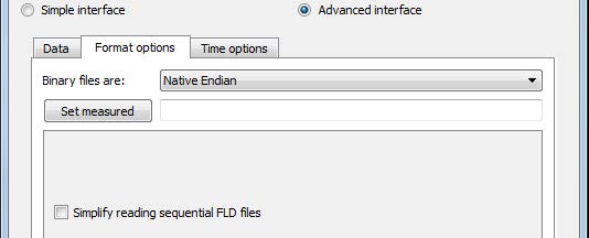 |
|
Simplify reading sequential FLD files |
Creates a location map of the FLD file data that is used to facilitate subsequent finding of data within the file. |
See Read Data
The following topics are included in this section:
Description
Reads .stl files and .xct exec files.
Overview
Description
This reader will load STL files (either ASCII or binary).
Note: STL files consist only of surfaces (triangles) and have no associated variables.
Usefulness
STL geometry format is widely compatible with a number of codes.
Multiple STL files geometries can be created to represent scenery or background, then read
in and scaled (using the -scaleg option) as a separate case to add to the
presentation of your existing model results in EnSight.
Usage
The STL reader can read in an individual .stl file, or it can read in an exec file so that more than one STL file can be included in the same case.
Limitations
The current reader does not allow the coloring of each facet, nor does it allow coloring of each part, and just skips over color statements in the file.
STL Binary File Format
If the file is a binary STL (.stl) file, then it must contain exactly one part.
STL ASCII File Format
If the file is an ASCII STL (.stl) file, then it can contain one or multiple parts. If you wish to read in multiple files
Single file multipart ASCII format is as follows:
solid part1
...
endsolid part1
solid part2
...
endsolid part2
Simple Exec File Format
An exec file (.xct) is used to read in multiple STL files into one case. Because binary STL can contain only one part, if you wish to read in more than one binary STL file into a single case, then you must use an exec file. ASCII STL files with one or multiple parts can be read in to a single case using the exec file. An exec file can read in binary and ASCII files together into a single case. This exec file is a very simple ASCII file that must conform to the following:
All lines must begin in column 1
No blank or comment lines allowed
If the STL filenames begin with a /, it will be treated as absolute path. Otherwise, the path for the exec file will be prepended to the name given in the file. Therefore, relative paths should work.
line 0: numfiles: N (where N is the no. of
            files)
line 1-n: stlfilename1
. . .
. . .
stlfilenameN
Example Simple Exec File
numfiles: 3
CASTLE.STL
bincastle.stl
test.slp
Rigid Body Motion Exec File
Release 2.1 of the STL reader includes the added ability to link each STL part with a rigid body transformation file to allow the STL part to rigidly translate and rotate over time. The rigid body motion Exec file has additional columns that contain the Euler Parameter filename (see Euler Parameter File Format), the transformation title in the Euler Parameter file, and a units scale factor (This is used to scale the translations, not the geometry. Scaling of the geometry is accomplished in the Part Feature Panel.). The rigid body version of this Exec file requires quotes as shown around the strings and values of the file lines.
Example 2.15: Rigid Body Motion Exec File
numfiles: 3
"CASTLE.STL" "motion.dat"
              "CASTLE" "1000.0"
"bincastle.stl" "motion.dat"
              "BCASTLE" "1000.0"
"test.slp" "motion.dat" "TEST"
              "1000.0"
And if an additional offset is needed to the CG, add these in 3 more columns
Example 2.16: With Additional Offset
numfiles: 3
"CASTLE.STL" "motion.dat"
              "CASTLE" "1000.0" "1.35" "2.66" "0.0"
"bincastle.stl" "motion.dat"
              "BCASTLE" "1000.0" "-2.45" "1.0" "-2.0"
"test.slp" "motion.dat" "TEST"
              "1000.0" "60.2" "23.4" "0.0"
You can also add a rotation order and yaw, pitch, and roll values on each of the file lines if the coordinate system must be re-oriented. These additional columns follow the same format as those in the EnSight Rigid Body (.erb) file.
See EnSight Rigid Body File Format).
README
See the following file for current information on this reader.
$CEI/ensight251/src/readers/stl/README
Simple Interface Data Load
Load your geometry file (typically named with a suffix .stl or .xct) using the Simple Interface method.
Advanced Interface Data Load
Load your geometry file (typically named with a suffix .stl or .xct) using the Advanced Interface method.
|
Data Tab |
|
|
Format |
Use the STL format. |
|
Set geometry |
Select the geometry file (typically .stl or .xct) and click this button |
|
Set results |
As of version 8.0.7(h) this field is activated to allow flags
to change reader behavior. In order to truncate the float values put in a tolerance
value and the reader will retain only to the designated significant digit. This can
be used to eliminate duplicate node problems due to round off error. Put in the
keyword |
|
Format Options Tab |
|
|
Set measured |
Select the measured file and click this button. |
See Read Data
The following topics are included in this section:
Description
This reader is unique in that it does not actually read geometry/variable data from the disk. Rather, it is designed to synthesize geometry/variables based on commands read in from a file or options chosen interactively in the Data reader dialog. The Synthetic reader can create transient or static geometry comprised of spherical and/or cube parts(s) with an arbitrary, user-defined number of elements (of user-chosen element type), that varies linearly over a user-chosen number of timesteps as well as any number of scalar, vector, or constant variables.
Note: It may not appear in your pulldown list of readers by default: to see this reader, go to Edit → Preferences → Data → Synthetic to make this reader available.
The most common usage is to interactively choose the Synthetic reader and to enter a sample filename in the data field (data reader dialog requires an entry in this field), and to toggle on the Advanced interface, and to interactively choose values in the Format options. These interactive sessions can be saved as command files to be rerun later, or session files to be reloaded later. More rare, is to hand-edit a synthetic options (.svn) file with specific entries, and then the load in the .syn file that will provide the input for generation of the dataset.
Usefulness
Because the synthetic reader does not read the geometry nor variable data from disk, it is useful for measuring EnSight performance separated from EnSight I/O. Further, the Synthetic reader is compatible with all of EnSight's parallel capabilities [SOS, Enterprise (formerly HPC+), threading]. As such, it is useful for measuring graphics hardware card performance by creating and controlling arbitrarily large numbers of polygons to be rendered by the client graphics card. Also, it is useful for supplying known models (size and element type) to quantify the benefits of parallel computing (threading) performance, as well as parallel server (SOS) performance, as well as parallel rendering performance. Further, in Compatibility mode (one of the user options), the synthetic reader is useful for comparing current versions of EnSight 2025 R1 to previous versions of EnSight. In addition, with the power of the EnSight calculator and the simplicity of the geometry the synthetic reader is a useful tool for verifying and validating the calculator functions over the range of element types supported by EnSight.
Finally, the synthetic reader eliminates the need for transmitting extremely large datasets for testing purposes. Since geometry is generated from commands, arbitrarily large geometries for testing can be sent via email in the form of tiny .syn files, or in .enc command files that contain the format options for creating the gigantic dataset.
Usage
The synthetic reader must have text in the file field, even if it is sample text because of EnSight requirements (in which case it will ignore the sample text) or it can read in a .syn file so which will contain a simple list of options for auto-generating the geometry, timesteps, variables, etc.
Limitations
The current reader only allows a subset of the EnSight element types, and all parts currently contain only one element type. Elements of type TRI03 are used to create a surface mesh on the outer boundary of the sphere or the cube part(s) or the plane part(s). Volume elements create a 3D volume of the sphere or cube part(s). And QUAD04 elements create a series of layers in the cube part(s).
Elements
There are three part types: Spheres, Cubes and Planes. If you choose Tri 3 then the surface of both the sphere and cube part(s) are meshed using this element type. If you choose another element type, then the sphere(s) are meshed using the Hex 8 element type, and the cubes are meshed using the element type. For example, choose the Point element type and the Cube nodes become point elements. Choose the Quad4 and the cube becomes a series of xy planes meshed in Quad 4 elements. Similarly choose Tet 4, Penta6, Nfaced Polyhedral, or Structured Hex and the cube part's hex elements are converted into these supported 3D element types. Planes must use Tri 3 or Quad 4 elements only. Unfortunately a large number of element types are still unsupported: Bar 2, Bar 3, Tri 6, Quad 8, Tet 10, Pyr 5, Pyr 13, Penta 15, Hex 20, and Nsided Polygon. Choose an unsupported element type and the cubes and spheres are meshed using Hex 8 elements and a warning message is sent to the server console.
Plane Parts
Plane parts are unique as follows. Each part has one plane. Plane parts are all normal to the Z-axis and appear back to front uniformly distributed along the Z-axis from Z=0 to Z=1. Planes interpolate between the beginning and ending number of elements (which are elements per part). At earlier timesteps, parts with higher part number are effectively given zero nodes and zero elements. As you proceed through time, parts are allowed to have elements. This allows the appearance of parts as you proceed through time, from back to front, of increasingly dense numbers of elements (when the ending number of elements is higher than the beginning) resulting in an exponential increase in the number of elements, for example, for graphics testing. If the Spread is set to Legacy, then the planes x and y centers are exactly aligned. A different Spread will add some random scatter to the x and y centers. If the number of plane parts is less than the number of servers then the part will be assigned to the server by part number. If there are more parts than servers, then a round-robin approach will apply.
Variables
Scalar and vector variables alternate as nodal and elemental, respectively. The first scalar variable (nodal) is a nodal deformation scalar, and the second variable (elemental) is simply the element index. The first vector variable (nodal) is a spiraling vector simulating a swirling flow spiraling inward and downward. The first two constant variables are the number of nodes and the number of elements, respectively. Other variables will be added as needed/requested. Finally user variables can be added using the calculator (for example, a quadric dependent on the Coordinates).
Transient
If one timestep is chosen the dataset is static. If more than one timestep is chosen, and the dataset is in compatibility mode, then the dataset is changing connectivity. If compatibility mode is off and the begin number of elements is the same as the ending number of elements, then the dataset is changing coordinates only.
README
See the following file for current information on this reader.
$CEI/ensight251/src/readers/synthetic/README.txt
Simple Interface Data Load
For auto-generating a dataset, simply load a synthetic file (typically named with a suffix .syn) using the Simple Interface method. For interactive use, toggle on the Advanced Interface Data Load.
Advanced Interface Data Load
Toggle on the Advanced Interface for interactive creation of your dataset. Then, put a junk filename in the data file name field (for example, dd) because the EnSight dialog requires a filename (even a bogus one) and then go directly to the Format options tab to control your geometry and variable generation. Interactive creation of your data requires the Advanced Interface method.
|
Data Tab |
|
|
Format |
Choose the Synthetic format. If this format is not available in this pull down list, then go into your preferences under the data tab and make this reader available. |
|
Set (Optional) |
Optionally choose a .syn file. Or, for interactive use, enter a fictitious filename (required to be non-empty by the dialog) and then toggle on the Advanced Interface and go to the Format options tab to design your geometry, variables, etc. |
|
Format Options Tab |
|
|
Set measured |
Select the measured file and click this button. |
|
Verbose mode |
Toggle this ON to get more output, useful for debugging purposes, output to the console. Default is OFF. |
|
Use ghost elements |
Toggle this on to create ghosts between the boundary shared by SOS servers. If running EnSight in SOS mode, then the geometry is automatically allocated evenly to each of the servers. Toggle this ON to use ghost elements between the servers. (Default is OFF). |
|
Long names |
Toggle this OFF to use simple part and variable names. Toggle ON to use long variable names. Default is ON. |
|
Compatible mode |
Toggle this ON and new options will be limited to retain compatibility with older versions of EnSight 2025 R1. Toggle this OFF to take advantage of new variables and new names, and other new features as they are added. Default is ON. |
|
Move Transient Parts |
Toggle this ON (Default) to randomly move parts' center of gravity linearly between randomly selected begin and end points through time. Toggle this OFF to cause the parts to remain stationary through time. Note: If you choose only one time step then this toggle is ignored and parts do not move. |
|
Element type |
Choose an element type. The following are allowable types but not all are supported (see above for details): Point, Bar 2, Bar 3, Tri 3, Tri 6, Quad 4, Quad 8, Tet 4, Tet 10, Pyr 5, Pyr 13, Penta 6, Penta 15, Hex 8, Hex 20, Nsided Polygon, Nfaced Polyhedral, and Structured Hex. (Default is Tri 3). Over time, more supported types will be added. |
|
Boundary ghosts |
Choose None, Convert, or Add for controlling ghosts around the outer perimeter of the cube(s) and sphere(s). Ghosts are useful for allowing EnSight to interpolate variable values rather than extrapolate them. Choose None to use NO ghosts around the outer boundary. Choose Convert to convert the outer boundary of cells to ghost cells. Choose Add to add another layer of cells all around the outer perimeter of the part(s) that are ghost cells. Default is None, so legacy command files should work fine. |
|
Spread out parts |
Created parts by default (legacy) are created only slightly off center. This has the effect of creating overlapping parts when multiple parts are created which is not useful if you want to see each part individually. This option spreads the parts out Little, Medium or Large amounts in the XYZ directions randomly so that the parts are overlapping a little bit, some and are mostly spread out, respectively. This is useful, for example, if you want to see the individual coloration on a large number of parts. |
|
Number of spheres |
Choose the number of spherical parts. Default 0 |
|
Number of cubes |
Choose the number of cube parts. Default 1. |
|
Number of planes |
Choose the number of 2D plane parts. Default 0. |
|
Number of elements start |
Starting number of elements at timestep 0 for each part. Default 1000. The reader will attempt to create parts containing roughly this number of elements using an odd number of elements in each orthogonal direction. If you choose 1000 and two cubes with Hex8 elements, and two sphere parts then your total number of elements will be roughly 4000 elements. In reality your cubes will be of dimension 9x9x11 for a total of 891 elements and your spheres will also have 891 elements because they are cubic elements mapped onto a sphere resulting in 3564 total elements. |
|
Number of elements end |
Ending number of elements at the last timestep for each part. If you choose 10000 and two cube and two sphere parts then your total number of elements will be 40000. Default 1000. |
|
Number of timesteps |
Choose the number of timesteps. 0 means static data. Default is 0. |
|
Part scaling factor |
This is used for scaling the part. Default is 1.0 |
|
Random number seed |
This is for shifting parts randomly around so they don't all overlap each other. Default is 0. |
|
Number of scalars |
Even scalars are nodal and odd scalars are elemental. Default is 0. |
|
Number of vectors |
Even scalars are nodal and odd scalars are elemental. Default is 0. |
|
Number of constants |
The first two constants are number of nodes in the dataset and number of elements in the dataset. Default is 0. |
.syn file format
The .syn file can contain the following text:
#!SYN_CASE 1.0
NUMBER_TIMESTEPS num
NUMBER_SPHERES num
NUMBER_CUBES num
NUMBER_ELEMENTS_START num
NUMBER_ELEMENTS_END num
PART_SCALE num
RAND_SEED num
USE_GHOSTS num
VERBOSE num
ELEM_TYPE {see list}
NUMBER_CONSTANTS num
NUMBER_VECTORS num
NUMBER_SCALARS num
LONG_NAMES num
Valid values for ELEM_TYPE:
Point
Bar 2
Bar 3
Tri 3
Tri 6
Quad 4
Quad 8
Tet 4
Tet 10
Pyr 5
Pyr 13
Penta 6
Penta 15
Hex 8
Hex 20
Nsided Polygon
Nfaced Polyhedral
Structured Hex
For legacy reasons, the former tri and hex keywords are also still supported.
These options map 1 for 1 with the options found in the data reader dialog under the Format options Tab.
Note: USE_GHOSTS, LONG_NAMES and VERBOSE are true if <num> is non-zero.
.syn File Example
The following example creates a 20 timestep dataset with 3 spheres and 2 cubes. Each sphere/cube will have 1M triangles. Each cube and sphere will have a diameter of 0.2 (and the centroid will be randomly placed inside of a 1.0x1.0x1.0 box).
#!SYN_CASE 1.0
NUMBER_TIMESTEPS 20
NUMBER_SPHERES 3
NUMBER_CUBES 2
NUMBER_ELEMENTS_START
            1000000
PART_SCALE 0.2
See Read Data
The following topics are included in this section:
Description
There are two Tecplot readers included with EnSight: Tecplot Binary and Tecplot_ASCII which read binary and ASCII Tecplot data.
TECPLOT Binary Reader Usage
The TECPLOT binary file format uses a Tecplot PLT file.
Tecplot ASCII Reader
A subset of the Tecplot 360 ASCII format is read using the Tecplot_ASCII reader. This is discussed below. In the format options tab of the data reader dialog, choose Debug to get extra output to the console if EnSight fails to read your ASCII file.
README
See the following directory for current information on these readers.
$CEI/ensight251/src/readers/tecplot/
Simple Interface Data Load
Load your Tecplot file (typically named with a suffix .plt or .plot or .dat) using the Simple Interface method.
Advanced Interface Data Load
Load your Tecplot file (typically named with a suffix .plt or .plot or .dat) using the Advanced Interface method.
|
BINARY |
|
|
Format |
Use the Tecplot Binary, or the legacy TECPLOT 7.x format. |
|
Set plot (or dat) |
This field should have the .plt name for binary data. Use a asterisk for transient multiple files (one timestep per file), filename*.dat |
|
Format Options Tab Tecplot BINARY |
|
|
Set measured |
Select the measured file and click this button. |
|
Tecplot Binary Other Options |
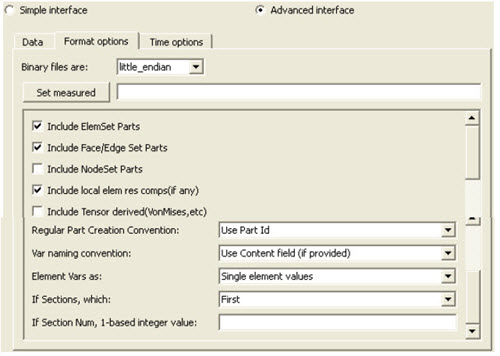 |
|
Include any Element sets defined. These are sets of full elements which are generally some logical subset of the total number of elements. Default is on. |
|
|
Include Face/Edge Parts |
Include any Face or Edge sets defined. These are some logical set of particular faces and/or edges of full elements. Default is off. |
|
Include NodeSet Parts |
Include any Node sets defined. These are generally the subset of nodes needed for the Element, Face, or Edge sets above. As such, they are generally not needed as separate parts, but can be created if desired. Default is off. |
|
Include local elem res comps (if any) |
Include the local stresses components, etc that are in the element's local system. A simple example is a bar (such as a truss element), which only has tension or compression in the element's axial orientation. Such an element would have an axial stress variable. Other elements would have appropriate result component variables. Default is on |
|
Include Tensor derived (VonMises, etc.) |
For tensor results, calculate scalars from the following derived results (principal stress/strains, and common failure theories): Mean Equal Direct VonMises Min Principal Octahedral Mid Principal
Intensity Max Principal Max Shear
By default, all 9 of these will be derived. You can control which are created by this toggle, with an environment variable. Namely, setenv ENSIGHT_VKI_DERIVED_FROM_TENSOR_FLAG n where n = 1 for Mean only 2
for VonMises only 4 for Octahedral only 8 for Intensity only 16 for Max Shear only
32 for Equal Direct only 64 for Min Principal only 128 for Mid Principal only 256
for Max Principal only 512 for all
or any legal combination. example: for VonMises and Max Shear only, use 18. Default is off |
|
Regular Part Creation Convention |
Parts will be created according to the following: Use Part Id - Part Id (this is the default) Use Property Id - Property Id Use Material Id - Material Id |
|
Var naming convention |
Use Content Field (if provided) - Variable names will be what is in the Content field, if provided. If not provided, they will be the VKI dataset name. This is the default. Use VKI dataset name - Variable names will be the VKI variable dataset name (which are reasonably descriptive). |
|
Element Vars as |
Single element values - Element results (whether centroidal or
element nodal) will be presented as a single value per element. Therefore will be
Averaged to node values - Element results (whether centroidal
or element nodal) will be averaged to the nodes without using geometry weighting.
Therefore will be Geom weighted average to node values - Element results (whether
centroidal or element nodal) will be averaged to the nodes using geometry weighting.
Therefore will be Ave to node values <by parts> - Element results (whether
centroidal or element nodal) will be averaged to the nodes without using geometry
weighting. Therefore will be Geom weighted ave to node <by parts> - Element results
(whether centroidal or element nodal) will be averaged to the nodes using geometry
weighting. Therefore will be |
|
If Sections, which: |
Which section will be used to create the variable First - The first section will be used (this is the default) Last - The last section will be used Section Num (below) - The section number entered in the field below will be used Separate Vars per Section - A separate variable will be created for each section. |
|
Section Num |
If the previous option is chosen to be Section Num, then the value in this field is the 1-based section number to use to create the variable. |
|
ASCII |
|
|
Format |
Use the or Tecplot_ASCII. |
|
Set plot (or dat) |
This field should have the .dat file name for ASCII data. Use a asterisk for transient multiple files (one timestep per file), filename*.dat |
|
Format Options Tab Tecplot ASCII |
|
|
Set measured |
Select the measured file and click this button. |
|
Tecplot ASCII Other Options |
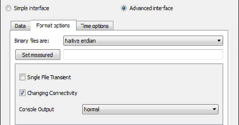 |
|
Single File Transient |
Toggle this ON to load a single file as transient data (default is OFF). If this toggle is ON, then the reader tries to find the SOLUTIONTIME keyword to identify the time value of a given part. If ZONE T= keyword is encountered prior to finding a SOLUTIONTIME keyword, then the reader tries to parse the Zone T contents to determine the time for that part. So the ZONE T must contain a parseable time value if there is no SOLUTIONTIME keyword. |
|
Changing Connectivity |
There is no meta-data in the Tecplot ASCII file indicating whether the connectivity changes over time. When this toggle is ON, then transient data is loaded as changing connectivity (coordinates and connectivity are read in at every timestep, which is the safe (but slow) assumption (default ON). This causes EnSight limitations, such as temporal calculations and temporal queries and inability to interpolate between timesteps. So if you know that your data doesn't change connectivity through time you can toggle this off. If you are wrong then EnSight may crash. |
|
Console Output |
If you want more information and detail about the file you are reading, choose Console Output Verbose. If you are having problems reading the file, choose Console Output Debug. The Console output is generated at the Server console window. Problem reports should include the Console output debug information. Note: Default is Normal which includes very little server console output). |
See Read Data.
The following topics are included in this section:
Reader Visibility Flag
By default, this reader is not loaded into the list of available readers. To enable this reader go into Edit → Preferences and click on Data and toggle on the reader visibility flag.
Reader vs. Translator
This reader is designed for files written before Vectis 3.6. For versions 3.6 or later, we recommend using the Ricardo v2e translator to convert the Vectis POST file to the EnSight format.
Pre-version 3.6 Description
This reader inputs either .tri or .pos datasets as follows
Single TRI file - Gives the CAD geometry, but no variables (If you must see this along with your POST data, will have to read it as a second case), for example, CYLINDER.TRI
Single POST file WITH NO *'s in the name - Gives the geometry and variables in the post file, including surface patches and particles.
Multiple POST files - Enter a filename WITH *'s in the name
Gives the geometry and variables in the post files, which match the asterisks in a sequentially increasing pattern (starts at 1, increases by 1).
Note: If your naming/numbering scheme is different than this, we require you to rename/renumber.
Query over time
Query node over time operation within EnSight will only work for cell variables on the cell part. Patch and drop variables will currently return all zeros.
Cell Variables
You may request cell variables on patch or droplet parts. The cell variable will be mapped onto them. BUT, be aware that any portions of the patches which are actually in the external cells will have zero values, because VECTIS doesn't contain that info directly. This leads to slightly streaked or blotched models which basically show the variable, but are probably not presentation quality. In order to eliminate this effect, neighboring cell information will need to be accessed - and at this time that work has not been done. Consider using EnSight's Offset Variable capability - it might be useful for certain models.
README
See the following file for current information on this reader.
$CEI/ensight251/src/readers/vectis/README.txt
Simple Interface Data Load
Load your Vectis file (typically named with a suffix .tri or .pos) using the Simple Interface method.
Advanced Interface Data Load
Load your Vectis file (typically named with a suffix .tri) using the Advanced Interface method.
|
Data Tab |
|
|
Format |
Use the Vectis format. |
|
Set tri/pos |
Select the vectis file (typically .tri or .pos) and click this button. This field should written by a Vectis version earlier than 3.6 |
|
Format Options Tab |
|
|
Set measured |
Select the measured file and click this button. |
See Read Data.
The following topics are included in this section:
Description
This reader is designed to read the VTK, VTU, VTS, VTR, VTI, VTP, VTM,PVTI, PVTP, PVTR, and PVTU file formats.
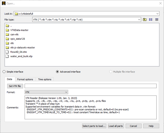
VTK
The VTK format is a legacy format containing both geometry and variable data.
VTU, VTS, VTR, VTI, and VTP
These formats are a Serial Grid format using an XML-based syntax containing both geometry and variable data. However, VTU uses an Unstructured Grid (vtkUnstructuredGrid), VTS uses a Structured Grid (vtkStructuredGrid), VTR uses a Rectilinear Grid (vtkRectilinearGrid), VTI uses a Uniform Image Grid (vtkImageData), and VTP uses polygonal data (vtkPolyData).
VTM
The VTM file enables you to pass in one filename that points to many spatially decomposed files, each containing a portion of the solution that was run in parallel. For example, the VTM file can contain multiple serial VTK, VTU, or VTS filenames, that were perhaps solved by multiple, parallel compute nodes. And, each of the VTK, VTU, or VTK files contains its own geometry and variables representing a spatial decomposition of the total solution at a given timestep.
For example, suppose you have transient data with two timesteps solved on four solver compute nodes. You might have the following files and sub folders:
file_0.vtm
file_1.vtm
./dir0/file_0_0.vtu, ./dir0/file_0_1.vtu, ./dir0/file_0_2.vtu, ./dir0/file_0_3.vtu
./dir1/file_1_0.vtu, ./dir1/file_1_1.vtu, ./dir1/file_1_2.vtu, ./dir1/file_1_3.vtu
Note: file_0.vtm and file_1.vtm each points to the geometry and variables at timestep 0 and 1, respectively. It is important to remember that file_0.vtm contains XML pointing to its four files using a local folder structure as shown below, so it is critical that the subfolder and file structure be maintained if the data is moved. Shown below are the spatially decomposed files for timestep 0 found in dir0.
dir0/file_0_0.vtu
dir0/file_0_1.vtu
dir0/file_0_2.vtu
dir0/file_0_3.vtu
PVTI, PVTR, PVTP, and PVTU
These are parallel XML based data files, which are designed for applications with multiple processes executing in parallel. The dataset does not contain real data, but instead only describes the structural information of the partitioned dataset. The dataset is divided into many files and stored separately. PVTI is the parallel version of the VTI format, PVTR is the parallel version of the VTR format, PVTP is the parallel version of the VTP format, and PVTU is the parallel version of the VTU format.
Transient
Since each file represents a single timestep, use an asterisk (*) to read in transient data. Loading the transient VTM file in the example above would require picking one of the .vtm files (so that it appears in the load field) and then typing in an asterisk in place of the number: file*.vtm.
SoS
The VTK reader supports parallel reading of the parallel VTM, PVTU, PVTP, PVTR, and PVTI file(s) (see Use Server of Servers).
VTM, PVTU, and PVTP
Suppose you are running EnSight in Server of Server (SoS) mode and enter in file*.vtm to read in transient data. If you have the same number of servers as files then each file is assigned to one server. In the above example, if you have four servers, then at timestep 0, the first server will read only the data contained in dir0/file_0_0.vtu. When you change time to timestep 1, the first server will now read the data from dir1/file_1_0.vtu. Similarly for the other servers, so that each server is reading spatially decomposed data completely separately from the other servers.
If you have less servers than files, then some servers will be assigned more than one file to read based on file sizes for efficient allocation of resources.
Currently the VTK reader does not support more servers than files for VTM, PVTU, and PVTP.
PVTI and PVTR
The servers will re-partition the image or rectilinear grid according to the number of servers given. There is no limit on the number of servers. However, since each server needs extra image/grid layers on the boundary to create hexahedral elements, the upper bound for optimal number of servers still exists to achieve the best performance.
Limitations
Previously, the reader did not support n-faced, 3D polyhedral elements in any of the formats (they were simply skipped and would result in holes in your geometry). Now, the 3D polyhedral elements are officially supported.
Simple Interface Data Load
Load your file (typically named with a suffix .vtk, .vtu, .vtm, .vts, .vtr, .pvti, .pvtr, .pvtp or .pvtu) using the Simple Interface method.
Advanced Interface Data Load
Load your file (typically named with one of the above suffixes ) using the Advanced Interface method.
|
Data Tab |
|
|
Format |
Use the VTK format. |
|
Set vtm, vtu, vts, vtk, vtr, pvti, pvtr, pvtp, pvtu |
Select the VTK file (typically .vtk, .vts, .vtr, .vtu or .vtm) and click this button. Use file*.vtk, file*.vts, etc. (where the asterisk (*) replaces the number) for transient datasets. Each file will represent one timestep. Alternatively, you can select .pvti, .pvtr, .pvtp, or .pvtu files. |
See Read Data.
The following topics are included in this section:
Description
Reads eXtensible Data Model and Format files (.xmf files).
This reader is based on the XDMF2 library from https://www.xdmf.org.
The reader can handle most mesh types in XDMF except XDMF_MIXED (unstructured grids made of mixed types).
It does not handle the XDMF_POLYGON type.
Structured meshes are converted to unstructured form automatically by the reader. The reader supports variables of type:
XDMF_ATTRIBUTE_TYPE_SCALAR
XDMF_ATTRIBUTE_TYPE_VECTOR
XDMF_ATTRIBUTE_TYPE_TENSOR
With centering:
XDMF_ATTRIBUTE_CENTER_CELL
XDMF_ATTRIBUTE_CENTER_NODE
The reader can handle Tree grids. The reader does automatically decompose datasets for server of server mode (SOS) based on Tree grids. The various grid blocks are distributed round-robin over the servers. Grids that are not Tree grids will all be read on the first server.
The reader allows the user to pass a filename using a wildcard (* or ?) to select a collection of .xmf files. The reader assumes that each .xmf file contains a separate time step. Some checks are made to verify that each file has the same structure and variables, but the checks are not complete. Likewise, some basic checks are made for grids defined by reference. If all but one file has its grids' geometry or topology by reference, the reader will assume that they can be reused for other time steps. This allows for more efficient reading of time-invariant meshes.
The reader can also be passed a file in the schema:
<?xml version="1.0" ?>
<Xdmf>
<Dataset>
<File Name=".xmf file" [Time="unknown"]/>
<Template Name="sprintf for .xmf files" [Start="1"] [Step="1"] [Count="1"]
[TimeStart="unknown"] [TimeStep="1.0"]/>
</Dataset>
</Xdmf>
This defines a collection of files by specific names. These can be
via individual names or via a printf -style
filename template and associated start, step and count values. The file may also contain
time step values for each file (in the case of a
printf -style template, the values are generated).
Note: If a file has an <Information
Time=""/> element, that element will supersede the value specified
here.
Simple Interface Data Load
Load your file (typically named with a suffix .xmf) using the Simple Interface method.
Advanced Interface Data Load
Load your files using the Advanced Interface method.
|
Data Tab |
|
|
Format |
Use the XDMF2 format. |
|
Set xmf |
Select the file (typically .xmf) and click this button |
|
Format Options Tab |
|
|
Verbose mode |
Provide more output to the console to track progress and perhaps understand reader problems. |
|
Enable Data Freeing |
Attempts to free memory as quickly as possible (default ON). |
|
Flatten Grid into Separate Parts |
Controls whether to use only the top level XDMF grids (which can be a collection of grids) to create parts or to create a part for each grid. When toggled ON, EnSight will make each grid into a separate EnSight part (default OFF). |
|
Set measured |
Select the measured file and click this button. |
See Read Data.
The following topics are included in this section:
Description
Reads eXtensible Data Model and Format files (.xmf files).
This reader is based on the XDMF3 library from https://www.xdmf.org. The underlying XDMF3 library reads the vast majority of files written with the older XDMF2 library. Contact support if one of your older files cannot be loaded with the XDMF3 reader.
Supported data types
The reader can handle all mesh types in XDMF, including mixed unstructured grids, time-varying grid collections, and spatial grid collections.
The reader does not currently handle the XDMF_POLYGON type in any grid.
The reader supports variables of type:
XDMF_ATTRIBUTE_TYPE_SCALAR
XDMF_ATTRIBUTE_TYPE_VECTOR
XDMF_ATTRIBUTE_TYPE_TENSOR
With centering:
XDMF_ATTRIBUTE_CENTER_CELL
XDMF_ATTRIBUTE_CENTER_NODE
The reader supports XDMF mesh labels.
One limitation of the XDMF3 reader is its inability to automatically identify time-invariant datasets as such. The reference-counting method used with the XDMF2 library is no longer possible. Therefore, the XDMF3 reader identifies all grids as time-varying and connectivity-varying, even if the underlying data is not.
Parallelism
The reader automatically decomposes grid collections for parallel operation. The various grid blocks are distributed in a round-robin fashion over the servers. Grids that are not collections will all be read on the first server.
The reader allows the user to pass a filename using a wildcard (* or ?) to select a collection of .xmf files. The reader assumes that each .xmf file contains a separate time step. Some checks are made to verify that each file has the same structure and variables, but the checks are not complete.
Dataset Organization
An XDMF file is typically made up of several files. The intent of the XDMF library is to house lightweight data (for example,, mesh and variable definitions) in an ASCII XML file and the heavyweight data (for example, coordinates, mesh connectivities, variable values) in a binary HDF5 file. The XML file references the HDF5 file.
In addition to this, the XML file may also reference other files, other XML files for mesh blocks, other XML files for other time steps, or even other HDF5 files. These additional XML files may themselves contain more references. An XDMF dataset is almost never contained in just a single .xmf file. Therefore, when one moves an XDMF dataset around, one must be careful to keep all of the files that comprise the data together in the same relative locations.
Simple Interface Data Load
Load your file (typically named with a suffix .xmf) using the Simple Interface method.
Advanced Interface Data Load
Load your files (typically named with a suffix .xmf) using the Advanced Interface method.
|
Data Tab |
|
|
Format |
Use the XDMF3 format. |
|
Set xmf |
Select a file (typically .xmf) and click this button |
|
Format Options Tab |
|
|
Enable Data Freeing |
Attempts to free memory as quickly as possible (default ON). |
|
Flatten Grid into Separate Parts |
Controls whether to use only the top-level XDMF grid collection to create parts or to create a part for each subgrid. When toggled ON, EnSight will make each subgrid into a separate EnSight part (default OFF). |
|
Sets specify ghost elements |
The XDMF format standard does not define how to specify ghost elements. Some users employ XDMF Sets for this, including all ghost elements in a Set. But other users employ Sets for other purposes. Turning this option on (default OFF) instructs the reader to consider any element defined in any XDMF Set as a ghost element. |
|
Verbosity |
No messages (silent) Errors only Main progress All messages (debug) |
See Read Data.