In this validation study, it is shown that the combination of the Discrete Element Method (DEM) with Archard's wear law is effective for simulating wear in mill cases. The wear rate in the DEM model is significantly higher than the experimental rate, and the entire wear process was simulated within a few mill revolutions. Based on the Lethabo mill described by Kalala (2008)[8], this validation case highlights the accuracy of mill wear simulation using the DEM method.

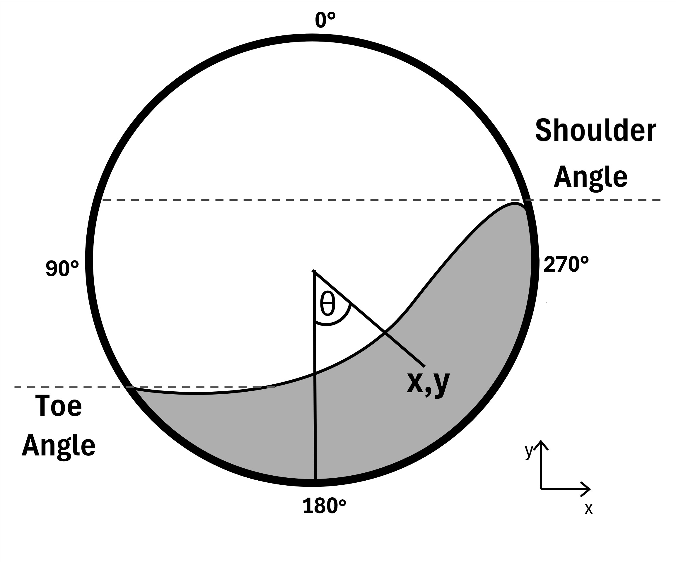
The Shoulder, Toe and angles (Figure 2.10: Schematic View of the Load Angles ) were compared between the simulation described by Kalala (2008)[8] and the simulation performed in Rocky DEM and show good agreement ( Table 2.6: Comparison of Load Angles between Kalala (2008) and Rocky Simulation).

Figure 2.10: Schematic View of the Load Angles

Table 2.6: Comparison of Load Angles between Kalala (2008) and Rocky Simulation

Simulation Profile	Shoulder Angle (Degrees)	Toe Angle (Degrees)	Angle (Degrees)
Figure 2.11: Kalala (2008) Simulation Load Angles	303	128	34.68
Figure 2.12: Rocky Simulation Load Angles	295	132	36.05
Relative Error (%)	-2.6	3.1	3.9

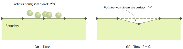
The Archard wear model is a shear-based model that correlates volume losses with the work due to friction forces (Figure 2.13: Application of the Archard wear model in Rocky DEM simulation. ). This model has been extensively correlated with a wide variety of materials and is frequently used by the mining industry to simulate wear. The following equation shows the application of the Achard Wear Model in Rocky DEM simulation:

(2–5)

where:

The input parameters for this validation case setup are presented in Table 2.7: Validation case input parameters.

Table 2.7: Validation case input parameters.

Parameter	Value	Unit
Physical Model:
Gravity (Z)	-9.81
Wall Geometry (Lethabo_10mm_mesh):
Diameter	4267
Triangle Size	15
Material Density	7850
Young's Modulus	1e+11
Poisson's ratio	0.3	-
Shear Work Proportionality (Achard's Law)	5e-07
Motion Frames (Mill Rotation):
Motion Time	0 - 1000
Initial Angular Velocity	-15.7
Particle Properties (Ball):
Diameter	50	mm
Material Density	7850
Young's Modulus	1e+08
Poisson's ratio	0.3	-
Materials Interactions (Ball Material X Mill Material):
Static Friction	0.2	-
Dynamic Friction	0.2	-
Tangential Stiffness Ratio	1	-
Contact Stiffness Multiplier	1	-
Restitution Coefficient	0.4	-
Materials Interactions (Ball Material X Ball Material):
Static Friction	0.2	-
Dynamic Friction	0.2	-
Tangential Stiffness Ratio	1	-
Contact Stiffness Multiplier	1	-
Restitution Coefficient	0.5	-
Solver Parameters:
Simulation Duration	110
Time Interval	0.5
Wear / Start	7.6
Geometry Update Interval	0.005

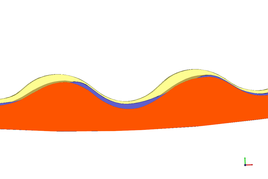
The experimental geometry was modeled based on the coordinates provided by Kalala (2008)[8]. After running the Rocky case as specified, the results can then be compared to the experimental values. This validation case demonstrate that such a modeling scheme still maintains reasonable accuracy in the geometry volume compared to experimental measurements, as we can see in Table 2.8: Comparison between the experimental and simulation geometry volume.

Table 2.8: Comparison between the experimental and simulation geometry volume.

Geometry	Volume ()	Relative Error (%)
Unworn reference	0.1131	-
Worn Experimental	0.0967	-
Worn Rocky simulation	0.0956	-0.8

It is also possible to verify that the wear profiles between the experimental geometry and simulation are similar (Figure 2.14: Comparison between profiles: Unworn reference (Yellow), Worn Experimental (Purple) and Worn Rocky simulation (Orange). ).

Figure 2.14: Comparison between profiles: Unworn reference (Yellow), Worn Experimental (Purple) and Worn Rocky simulation (Orange).