


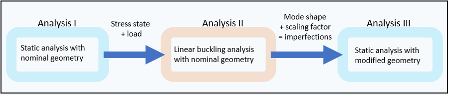
The suction-pile simulation involves three sequential analyses shown in the flow diagram below. For more details and the Workbench Project Schematic, see Figure 58.20: Workbench Project Schematic .
The example problem is organized to discuss each of the three analyses in the suction-pile simulation. The boundary conditions, loading, and results are described in the following sections for each analysis:
A nonlinear static analysis with nominal geometry is performed. The analysis accounts for a specific loading history to obtain a loading and stress state suitable for use in the subsequent buckling analysis. The following topics are discussed:
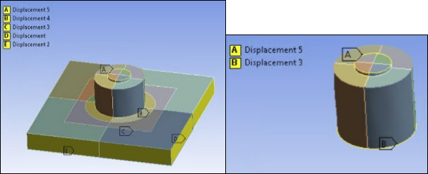
The following figure shows the displacement boundary conditions imposed for the nonlinear static analysis with nominal geometry. The bottom nodes of the soil and suction-pile skirt are fixed in the vertical (global Z) direction. Displacement in the perpendicular direction (global X and Y normal to the faces) is restricted on all four sides of the underground model. Displacement in the horizontal direction is also restricted on top outer ring of the suction pile.
Loading occurs over four steps:
An initial in-situ earth pressure is generated by applying a gravitational
acceleration of  to the soil in the vertical direction. A command Snippet
is used to apply gravitational acceleration to the individual bodies, where
ELEM_SOIL is a previously defined Named Selection that includes all geometry parts that make up the soil in the
model.
to the soil in the vertical direction. A command Snippet
is used to apply gravitational acceleration to the individual bodies, where
ELEM_SOIL is a previously defined Named Selection that includes all geometry parts that make up the soil in the
model.
CMACEL,ELEM_SOIL,,,9.81
The in-situ stress-state calculation leads to undesirable vertical deformations. To mitigate the problem, an initial stress state is applied, resulting in a nearly deformation-free initial state for the gravitational load step.
Typically, soil exists in an already-consolidated state. Initial
displacements due to at-rest loads are therefore unnatural and should be
minimized. The vertical stress state  varies linearly based on the soil depth.
  is determined via the soil density
  the gravitational acceleration
  , and the vertical height
  of each element:

The coefficient of lateral earth pressure  is defined as the ratio of horizontal- to vertical-stress
components. For a horizontally-retained, non-overconsolidated soil under
elastic loading conditions, the coefficient is defined via Poisson’s
ratio
is defined as the ratio of horizontal- to vertical-stress
components. For a horizontally-retained, non-overconsolidated soil under
elastic loading conditions, the coefficient is defined via Poisson’s
ratio  :
:

The horizontal stress components are then determined by:

The known stress state is applied as the initial state (INISTATE). The following command snippet is used to define initial state in the first load step.
!---------------------------------------
! Inistate soil

CMSEL,S,elem_outer1_soil
CMSEL,A,elem_outer2_soil
CM,elem_outer_soil,ELEM

accelz=-9.81

*dim,zone,char,1,2
zone(1,1)='outer'
zone(1,2)='inner'

!Loop outer/inner zone
*do,kk,1,2
    varzone=zone(1,kk)
    CSYS,0

    CMSEL,S,elem_%varzone%_soil
    NSLE,S,CORNER
    NSEL,R,LOC,Y,0
    *GET,mnloc_x,NODE,0,MNLOC,X
    NSEL,R,LOC,X,mnloc_x

    *GET,layer_nodes,NODE,0,COUNT
    layers=layer_nodes-1

    *DIM,layer_%varzone%_soil,ARRAY,layers,9
        !column1: item number
        !column2: upper z-coordinate
        !column3: lower z-coordinate
        !column4: item thickness
        !column5: item density
        !column6: item poisson's ratio
        !column7: INISTATE Cxx & Cyy
        !column8: INISTATE Czz
        *GET,min_elem_num,ELEM,0,NUM,MIN
        *GET,min_mat_num,ELEM,min_elem_num,ATTR,MAT
        *DO,ii,1,layers
            layer_%varzone%_soil(ii,1)=ii
            upper_node=NODE(mnloc_x,0,0)
            layer_%varzone%_soil(ii,2)=NZ(upper_node)
            NSEL,U,,,upper_node
            lower_node=NODE(mnloc_x,0,0)
            layer_%varzone%_soil(ii,3)=NZ(lower_node)
            layer_%varzone%_soil(ii,4)=layer_%varzone%_soil(ii,2)-layer_%varzone%_soil(ii,3)

            layer_cent=0.5*layer_%varzone%_soil(ii,4)
            elem_cent_depth=layer_cent-layer_%varzone%_soil(ii,2)
            *GET,layer_dens,DENS,min_mat_num,TEMP,elem_cent_depth
            *GET,layer_pois,NUXY,min_mat_num,TEMP,elem_cent_depth

            *if,layer_dens,eq,0,then
                *GET,layer_lat_pres,KXX,min_mat_num,TEMP,elem_cent_depth
                layer_%varzone%_soil(ii,9)=layer_lat_pres
            *else
                layer_%varzone%_soil(ii,9)=0
	     *endif

            layer_%varzone%_soil(ii,5)=layer_dens
            layer_%varzone%_soil(ii,6)=layer_pois
        *ENDDO

    INISTATE,SET,DTYP,STRE

    *IF,kk,LT,3,THEN
    upper_load=0
    *ENDIF

    *DO,ii,1,layers
        CMSEL,S,elem_%varzone%_soil
        NSLE
        NSEL,R,LOC,Z,layer_%varzone%_soil(ii,3),layer_%varzone%_soil(ii,2)
        ESLN,R,1
        layer_weight=layer_%varzone%_soil(ii,4)*layer_%varzone%_soil(ii,5)*accelz
        depth_weight=layer_weight/2+upper_load

        *if,layer_weight,eq,0,then
            lat_earth_pres=layer_%varzone%_soil(ii,9)
            layer_%varzone%_soil(ii,7)=-lat_earth_pres
            layer_%varzone%_soil(ii,8)=depth_weight
        *else
            k0=layer_%varzone%_soil(ii,6)/(1-layer_%varzone%_soil(ii,6))
            layer_%varzone%_soil(ii,7)=k0*depth_weight
            layer_%varzone%_soil(ii,8)=depth_weight
        *endif

        ! INISTATE command Cxx, Cyy, Czz, Cxy, Cyz, Cxz
        INISTATE,DEFINE,,,,,layer_%varzone%_soil(ii,7),layer_%varzone%_soil(ii,7),layer_%varzone%_soil(ii,8),0,0,0
        upper_load=layer_weight+upper_load
    *ENDDO
    *STATUS,layer_%varzone%_soil

*ENDDO
ALLSEL,ALL
INISTATE,WRITE,1,,,0,S

CMACEL,elem_soil,,,9.81
allsel,all
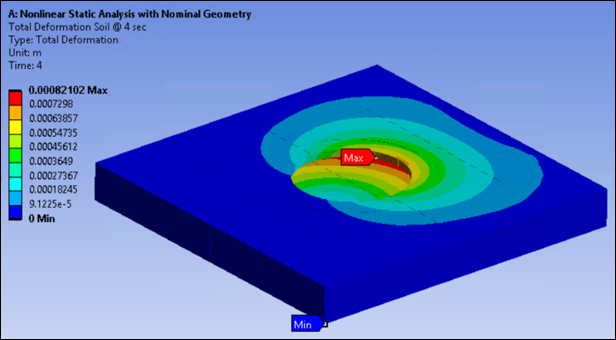
The following figure shows the resulting vertical-pressure distribution.
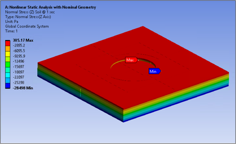
The initial at-rest pressure state is correctly applied while the soil structure retains its initial shape.
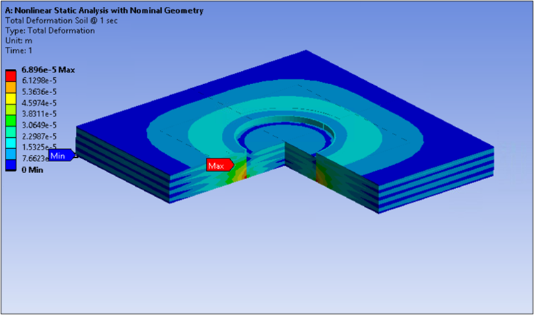
Marginal displacements (<0.5 mm) are acceptable due to unbalanced soil pressure inside and/or outside of the soil region and contact penetrations, and the following figure shows that the displacements are well under the marginal value.
A gravitational acceleration of  is applied to the suction pile using the following command
snippet, where ELEM_BUCKET is a previously defined Named Selection that includes all geometry parts that make up the suction pile
in the model.
is applied to the suction pile using the following command
snippet, where ELEM_BUCKET is a previously defined Named Selection that includes all geometry parts that make up the suction pile
in the model.
CMACEL,ELEM_BUCKET,,,9.81
allsel,all
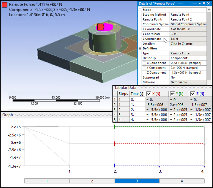
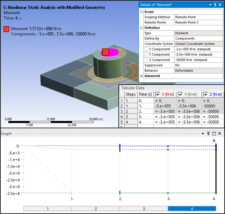
Forces caused by interaction with the upper structure are applied to the suction-pile top. Forces/Moments are distributed over the top of the pile using Remote Points, as shown in the following figures.
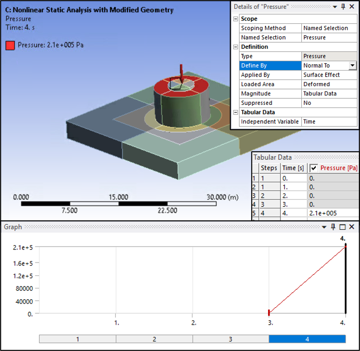
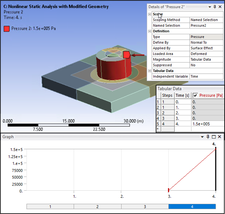
Suction pressure is applied on both the suction-pile skirt and cap. Constant pressure on the suction-pile skirt is assumed. The following figures show the applied suction pressure.
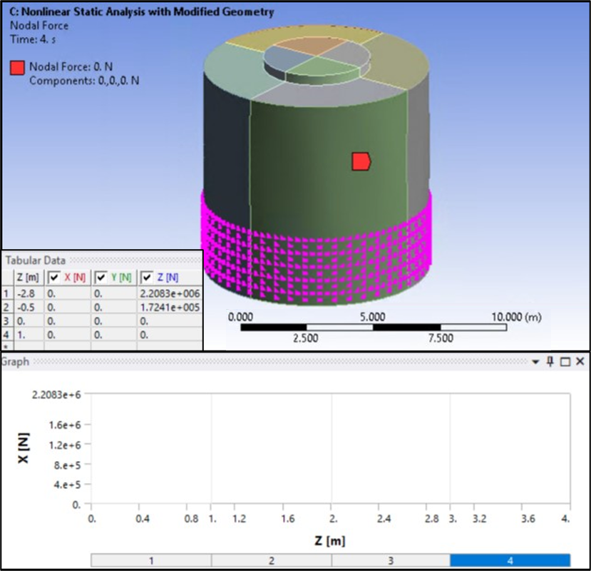
Assumed frictional forces are applied on the suction-pile skirt where the skirt interacts with the soil using a Nodal Force object.
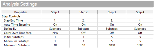
A nonlinear static analysis is performed. The in-situ stress state (load step 1) is calculated in a single substep. Load steps 2 through 4 are calculated with automatic time-stepping enabled.
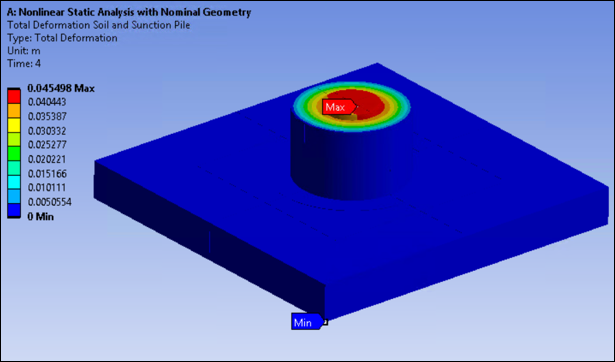
Initial-stress-state results are presented in Loading. The following figures show the results after load step 4.
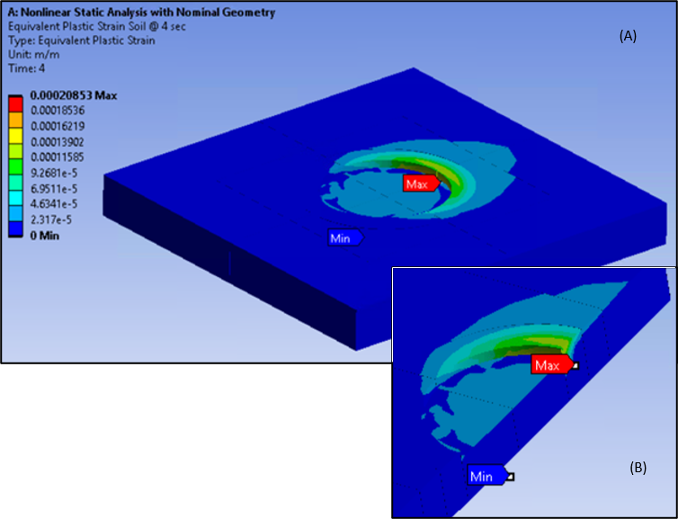
Loading on the suction pile leads to plastic strains in the soil as shown in the following figure. Plastic strains are distributed asymmetrically due to the asymmetrical loading in load step 3 and load step 4.
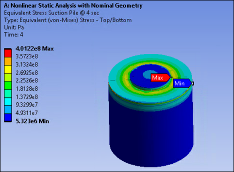
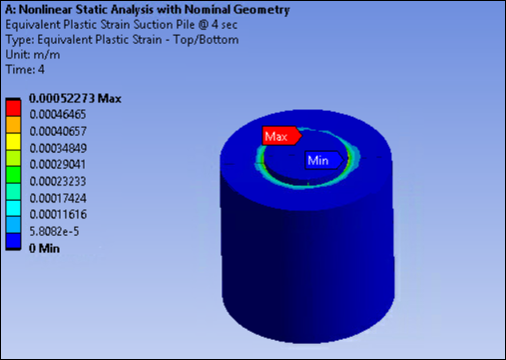
Strain on the suction pile causes plastic strains at the neck of the suction-pile cap shown in the following figure.
Following the nonlinear static analysis with nominal geometry, a linear buckling analysis with nominal geometry is performed to obtain potential stability modes related to the static loads. The results are used as the basis for defining imperfections.
Boundary conditions from the prior static analysis are used.
A final load state from load step 4 in the prior static analysis is used as a reference load.
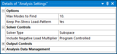
The linear buckling analysis is performed with the analysis settings shown below. Ten eigenmodes are calculated and expanded.
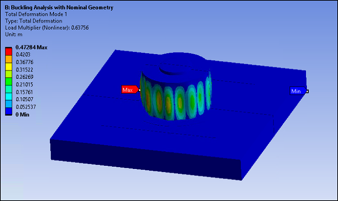
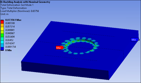
Ten eigenmodes were calculated during the buckling analysis. The resulting load factors range from 0.63756 to 1.1536. The following figures show the total deformation in the entire model and the soil calculated for the first buckling mode. The first buckling mode with a scaling factor of 0.135 is used to generate the structure imperfections for the modified geometry in the second static structural analysis.
A second nonlinear static analysis is performed using the updated geometry from the buckling analysis. To observe the influence of the added structural imperfections, the analysis uses the same loading from the first static analysis.
Boundary conditions from the first static analysis are used.
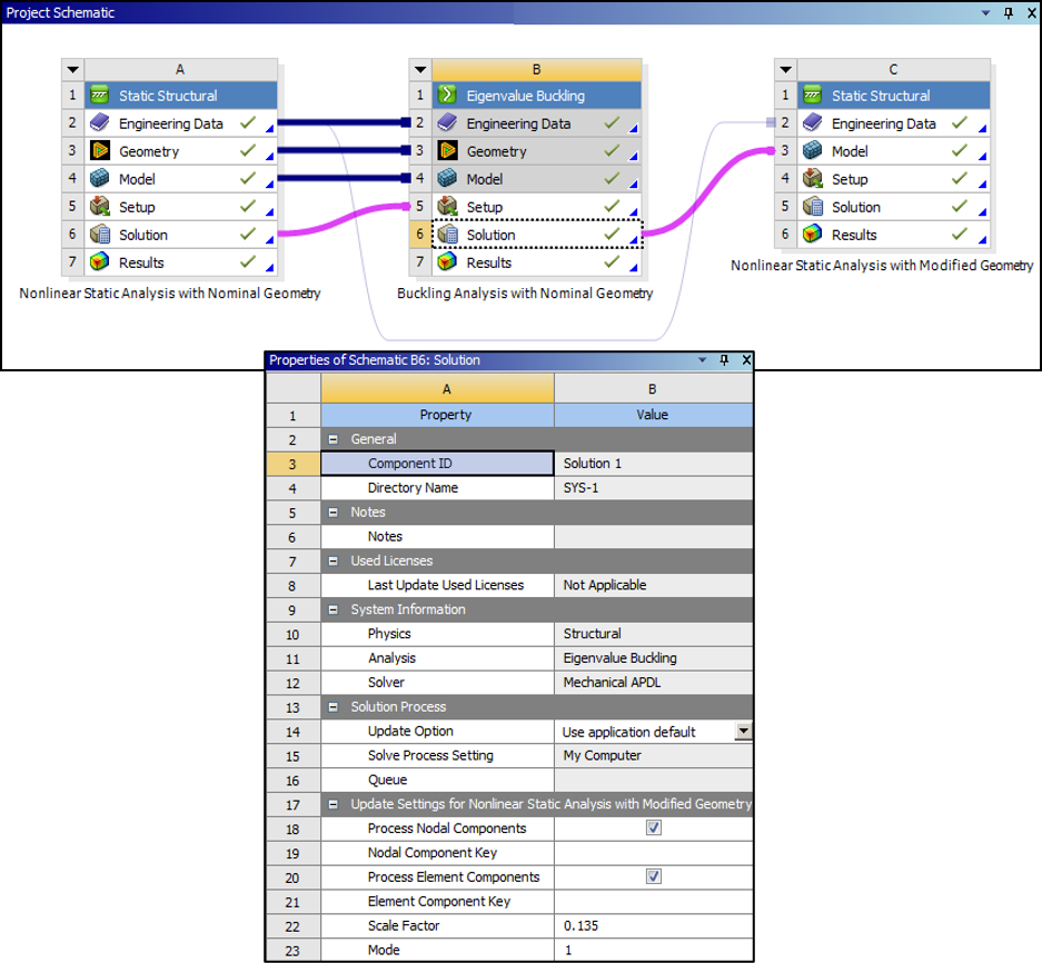
Loading for the second nonlinear static analysis is identical to the loading of the first static analysis. At the beginning of the analysis, however, the geometry is updated to account for imperfections based on the results of the buckling analysis. The Project Schematic below shows the three analyses, their links, and the settings on the solution cell of the eigenvalue buckling analysis system to update the geometry for the second static structural analysis with a 0.135 scaling factor.
A nonlinear static analysis is performed, similar to the first, but with the updated geometry.
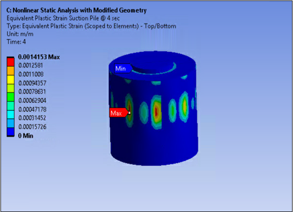
The following figures show the results after load step 4.
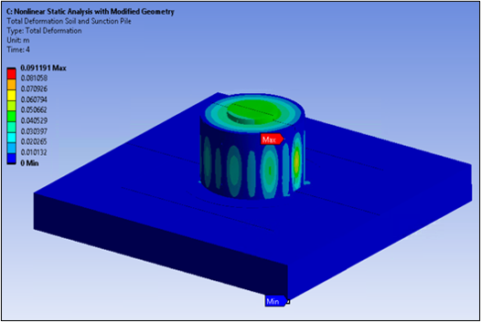
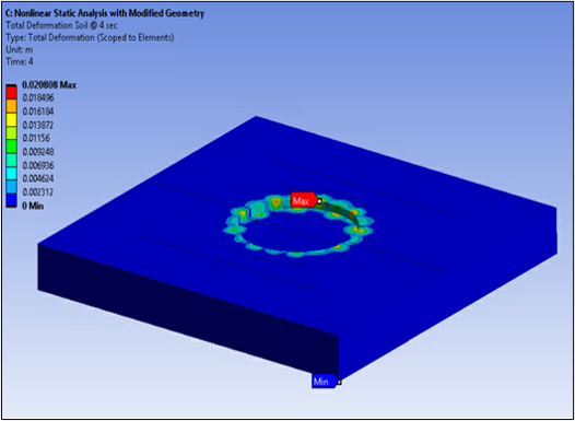
Figure 58.23: Equivalent Plastic Strains - Soil (A), Cross Section View (B), Second Static Analysis on Modified Geometry
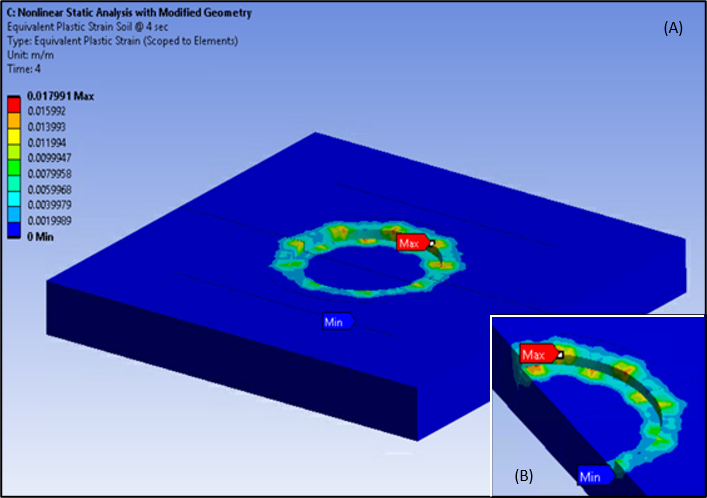
Compared to the static analysis results using nominal geometry, the analysis using the updated geometry with imperfections shows larger displacements and deformations on the suction-pile skirt, resulting in higher plastic strains.
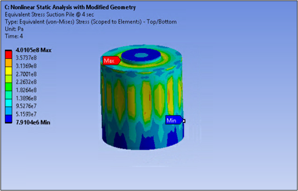
The suction-pile geometry without imperfections resulted in maximum plastic strains at the neck on the suction-pile cap. After including the imperfections, the same loading results in the critical region having moved from the suction-pile neck to the skirt.
Accounting for potential structural imperfections leads to qualitatively and quantitatively different results.