


The following examples demonstrate typical SMA-based applications with thermal loading:
The spinal vertebrae spacer is simulated via SOLID187 elements, and the spring actuator is simulated via BEAM188 and SOLID185 elements.
Approximately 20 percent of Americans between the ages of 20 and 64 have back pain problems,[1] most of which are associated with intervertebral disc (IVD) degeneration. In some cases, a degenerated IVD is surgically replaced with a spinal spacer inserted into the space between vertebrae, as shown in the figure below.
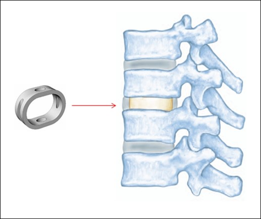
Spinal spacers restore disc space height, alignment, and the spine's ability to bear weight, any or all of which can be lost due to IVD degeneration. Finite element analysis of implant function can help improve the design and quality of the spinal spacer.
The following topics related to this example simulation are available:
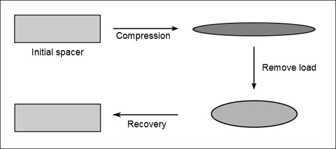
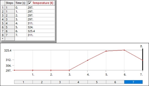
To simulate the function of a spinal spacer implant, the spacer is initially loaded at room temperature 297 K. The spacer is compressed from the top by a rigid surface to a thickness of 3.375 mm. The compression is then removed, and the spacer undergoes elastic recovery. To remove the residual strain, the spacer is heated to 326 K and then cooled to body temperature 311 K.
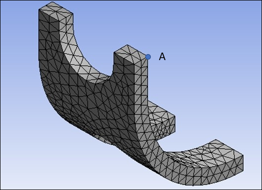
A 3-D geometry of the spinal spacer is created in Unigraphics, using dimensions found in Petrini 2005.[2] The geometry is imported into Mechanical and meshed with linear tetrahedron elements. Because the spacer is symmetrical, the model can be reduced to include only one quarter of the spacer, as shown below.
The spinal spacer analysis uses the following material properties:[2]
| Spinal Spacer Material Properties | |
|---|---|
| Elastic modulus for austenite phase (MPa) | 70,000 |
| Elastic modulus for martensite phase (MPa) | 70,000 |
| Poisson’s ratio | 0.3 |
| H (MPa) | 500 |
| R (MPa) | 120 |
| B (MPa ⋅ K-1) | 8.3 |
| T0 (K) | 311 |
| M | 0 |
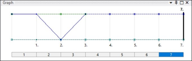
Symmetrical conditions are applied to the 1/4 model of the spinal spacer. A rigid surface contacts the top of the model, and a compressing displacement is applied to that surface. After the displacement is removed, a thermal load is applied to the whole model.
The nonlinear static analysis is performed with the Large Deflection property set to On in the Analysis Settings.
After the mechanical loading is applied, thermal loading is applied over three steps (4 - 6) for quicker convergence.
In step 4, the temperature is increased from 297 K to 311 K. Convergence is achieved quickly as this temperature is below T0.
In step 5, the temperature is again increased from 311 K to 324 K. The major phase transformation does not occur in this step, so convergence is again achieved quickly.
In step 6, the temperature is increased above 324 K, and the shape memory effect occurs, so convergence is slower.
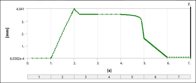
The following figure illustrates the displacement of the central point A (shown in Figure 40.3: Simulated model ¼ of Spinal Spacer).
The following figures show the deformation of the spacer at each step.

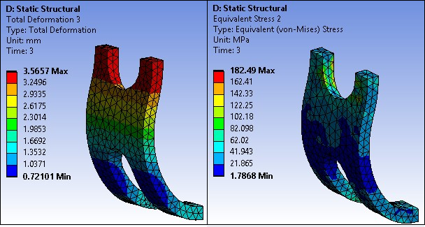
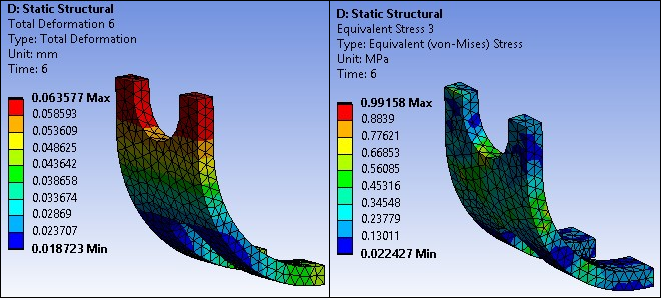
In step 2, the displacement is 4.04 mm and the stress is 594.2 MPa. After elastic recovery, the peak displacement decreases to 3.56 mm and the stress is 182.49 MPa. In the final step, displacement and stress approaches zero, indicating that the spacer has returned to its original shape.
The simulation accurately depicts the spacer under load (step 2), during elastic recovery (step 3), and at full recovery due to SMA thermal effects (step 6).
Because of their large-strain capabilities and high force-to-weight ratios, SMAs are widley used as compact, flexible actuators in a variety of industries. For example, SMAs can be used as combination sensor-actuators in thermal bridges for cryogenic coolers, variable-area exhaust nozzles for turbomachinery, and active clearance controls for blade shrouds. A prominent aircraft manufacturer has integrated SMAs into their variable geometry chevrons for engine noise control.
In this problem, a vertical helical spring is simulated to repeat its two-way motion due to the shape memory effect. The following related topics are available:
A vertical helical spring is simulated with shape memory effect using two different models, a BEAM188 element model and a SOLID185 element model.
The spring is loaded by a weight of 1830 N in the martensite state at a temperature of 250 K, then heated to 400 K. At the increased temperature, the spring lifts the weight. The spring is then cooled back to 250 K and stretches again. A repeatable, two-way motion occurs, as shown in the figure below.

The geometry of the spring actuator was created in DesignModeler with a wire diameter of 4 mm, a spring external diameter of 24 mm, a pitch size of 12 mm, with two coils, and an initial length of 28 mm, as shown in the following figure. See input files for links to download the .agdb files.
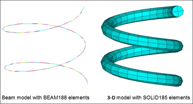
The corresponding finite element model is created using BEAM188 elements. A 3-D model is generated by extruding the initial finite element model and meshing with SOLID185 elements.
The following material properties,[3] typical of nitinol, are used in the spring actuator simulation:
| Material Properties for a Spring Actuator | |
|---|---|
| Elastic modulus for austenite phase (MPa) | 51,700 |
| Elastic modulus for martensite phase (MPa) | 51,700 |
| Poisson’s ratio | 0.3 |
| H (MPa) | 1000 |
| R (MPa) | 140 |
| B (MPa⋅K-1) | 5.6 |
| T0 (K) | 250 |
| M | 0 |
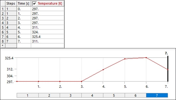
The top of the spring actuator is fixed, and the bottom is loaded with a weight of 1830 N. Displacements are constrained in the X and Y directions. After the spring is stretched by the weight at temperature 250 K, the temperature is raised to 400 K to lift the weight, and the is reduced back to 250 K to lower the weight. The following figures show the applied force and temperature histories.

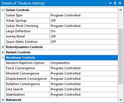
The nonlinear static analysis is performed with the Large Deflection property set to On and the Newton-Raphson Option set to Unsymmetric in the Analysis Settings (see figure below).
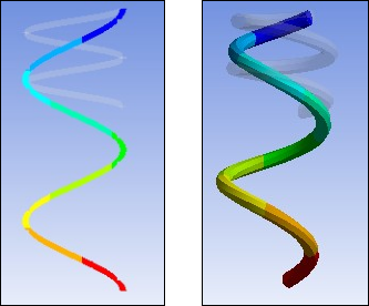
The spring actuator stretched by load W in step 1 is shown in the following figure.
The maximum displacement is 43 mm, greater than the original length of 28 mm.
In step 2, after heating with the shape memory effect, the spring actuator recovers to a maximum displacement of 10 mm. The deformation is in the martensite state to support the weight, as shown below.
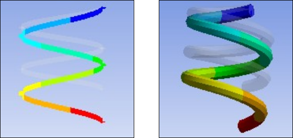
In step 3, after cooling to 250 K, the spring actuator stretches back to its original length:
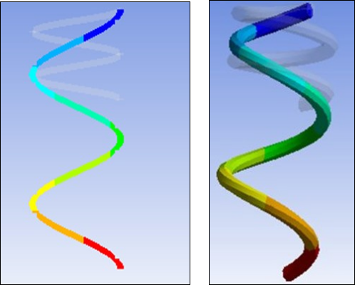
Results from the BEAM188 and SOLID185 models are compared. The following figure shows the displacement history of the actuator.
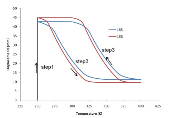
The displacement history indicates that the BEAM188 and SOLID185 models have similar results. The BEAM188 model is much more efficient, however, requiring about an hour to complete. In comparison, the SOLID185 model requires more than eight hours to complete.