


Orbital Plot maps are supported for Modal analysis systems. You can insert an Orbital Plot object to create a 360 degree visualization of the orbital plots. Orbital Plots are compatible both with and rotors.
For beam rotors, orbital plots are displayed for all the beam nodes. If using a 3D solid rotor model, the object will divide the centerline of the rotor into a user-defined number of points in order to visualize the orbital plot in those locations.
Create an Orbital Plot
Scoping is restricted to nodes and bodies and can be done using or . When scoping, the tool automatically detects whether the scope is a solid or beam rotor.
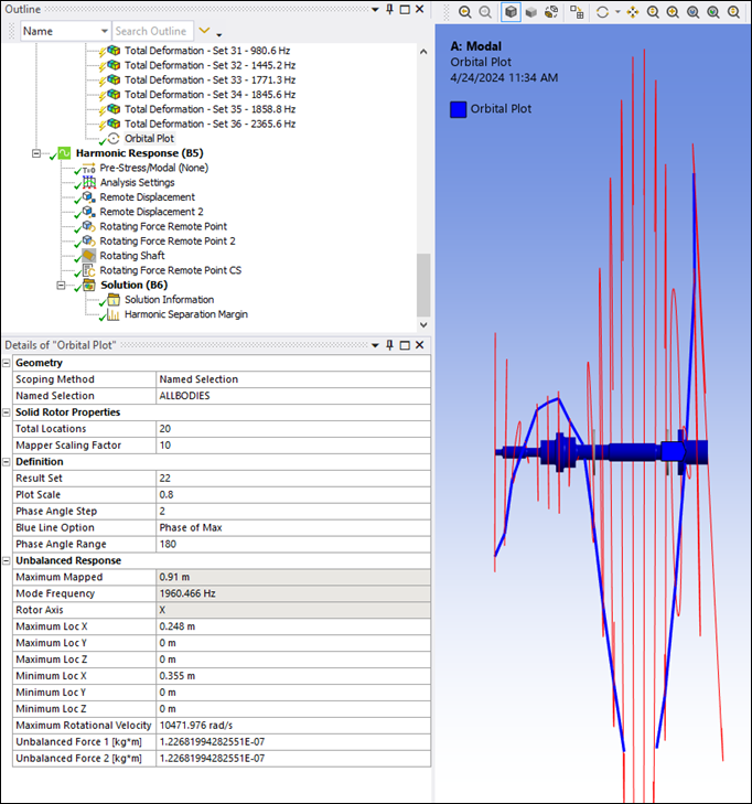
When selecting a solid rotor, the Solid Rotor Properties are displayed, so that you can define the Total Locations and Mapper Scaling Factor to use.
In the case of a solid rotor, the Rotordynamics tool solves the challenge of having a line of nodes in the centerline for hollow rotors (extrapolation) or coarse meshes without nodes in the centerline (interpolation).
A virtual set of nodes or locations is created along the rotor axis and the Ansys Data Processing Framework (DPF) RBF mapper is used to extrapolate or interpolate the modal results into those locations based on the surrounding nodal results.
The Total Locations property will divide the axis into the specified number of values to create the set of virtual nodes and will take surrounding values to perform the interpolation or extrapolation based on the Mapper Scaling Factor. The greater the Mapper Scaling Factor, the more values from the surrounding nodes will be taken.
The Result Set property sets the mode to use.
The remaining parameters help to the scale of the results for a better visualization as follows:
The Plot Scale varies the dimension of the plots.
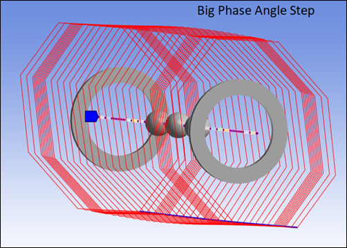
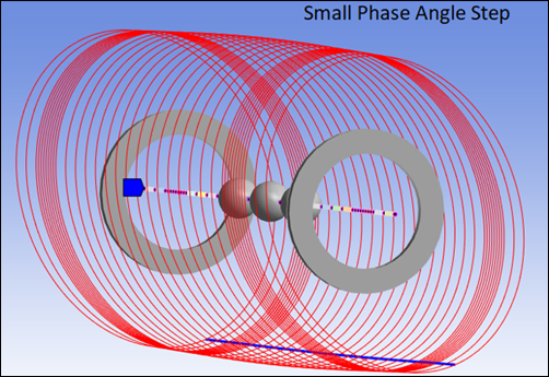
For Phase Angle Step, a smaller value leads to an orbital plot with smoother edges, since additional points are added in the circumferential plot (see below).
There are several options to display the connection between consecutive orbital plots (for example, the maximum value, or the intersection of the orbital plots with a specific plane), this is controlled by the Blue Line Option property in the Mechanical interface (see below).
Set the Blue Line Option to , , , , , , or to select the points of each 360 degree plot at which the blue line should be shown.
Phase Angle Range defines the range of the cutting plane in degrees.
Once all the properties are set, right-click the Orbital Plot and select the option to represent the orbital plots.
The Unbalanced Response panel for the Orbital Plot is populated with the corresponding Maximum and Minimum locations.
You must define Unbalanced Force 1 and Unbalanced Force 2 according to your specific standards or requirements.
You can also input maximum and minimum force locations to automate the creation of the forces. Once created, these locations can be modified using remote points.
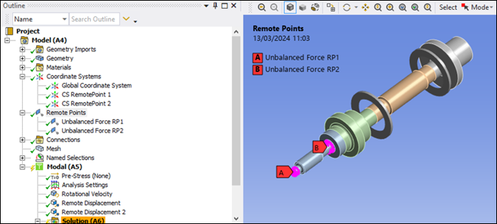
Add Example Unbalanced Forces
Once the Unbalanced Force example values are defined, you can right-click the Orbital Plot and select . Note that by default these loads are just examples and do not follow any specific norm. You must modify the location and values of these forces to unbalance the rotor according to the modal shape and your specific standards or requirements.
This action will automatically create the following objects:
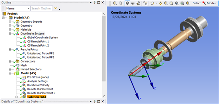
Two Coordinate Systems at the locations where the unbalanced forces are created.
Named Selections are created automatically by the tool by selecting the number of mesh nodes within a defined tolerance. The pre-set tolerance is −5e-3m and 5e-3m as the upper and lower bounding distance from the previously-created coordinate systems. You can adjust this tolerance in the worksheet as required.
Two Remote Points attached to the geometries at the location of the previously created Named Selections.
New objects are created In the Harmonic system for the Rotating Force Remote Points and the Rotating Shaft. Note that the added command snippet system is empty, and exists only to enable solution of the Harmonic system. Note also that when multiple Harmonic systems are present in the project, all of them will be populated with the previously mentioned objects. It is therefore suggested that you perform the unbalanced response analysis with only one Harmonic system in the project.
All the objects created can be easily modified to adapt to your specific requirements or standards.
Rotating Force Remote Point
The Rotating Force Remote Points added to the Harmonic system are located at the previously-created Unbalanced Force Remote Points, with the magnitude of the force defined in the Orbital Plot details panel.
This object adds the equivalent rotating force to that specific remote point location. When solving the Harmonic system, the corresponding Mechanical APDL commands are added to the ds.dat file to account for the rotating force.
You can redefine the remote point location (Geometry), rotational Global Axis, Force, and Phase as required.
Rotating Shaft
The rotating shaft must be scoped to bodies and the
Rotational Velocity Factor is always set to 1.
All geometries will rotate with the same defined rotational velocity.
When solving the Harmonic system, the corresponding commands are added to the input file (ds.dat) to confirm to the Mechanical APDL solver that all bodies are rotating with the same rotational velocity.