


Aqwa supports four types of cables, each with their own input requirements:
To add a Cable:
Select the Connections object in the tree view.
Right-click the Connections object and select Insert Connection > Cable, or click on the Cable icon in the Connections toolbar.
Select the Cable object in the tree view and set properties.
The Type of the cable (, , , or ) can be set in the details panel.
Cables may either be joined between two structures, between a fixed point and a structure, or between two fixed points via a pulley (only available for Linear Cables); this option can be changed via the Connectivity field in the Details panel. A cable cannot have both ends connected to the same structure. For the first two cases an End Connection Point must exist at the position of the end of the cable; this can be selected from a dropdown list of existing Connection Points defined on the structures. For the third case and End Fixed Point must be selected from a dropdown of existing Fixed Points. When the starting point is on a structure, you can define the start of the cable using Start Connection Point, which again is a dropdown list of existing Connection Points defined on the structures. When the starting point is a fixed point, a dropdown list of defined fixed points is shown.
Linear Elastic and Polynomial cables can be winched by adding a Cable Winch . All cable types can also have break conditions based on tension or time, defined by adding a Cable Failure object.
Set additional options in the Details panel for each cable type as described in the sections below. The extension of the cable and force applied depend on the Connectivity defined (the following information is not applicable to catenary cables):
For a cable attached between a structure and a fixed point
The extension of the cable, at any stage of the analysis, is calculated by subtracting the unstretched length from the distance between the position of the fixed point and the current position of the connection point on the structure.
The direction of this force is given by the vector going from the fixed point to the structure.
For a cable attached between two structures
The extension, at any stage of the analysis, is calculated by subtracting the unstretched length from the distance between the connection points on the two structures at the current position of the respective structures.
The direction of the force on a structure is given by the vector going between the two connection points. The forces on each structure will therefore always be equal and opposite and hence the selection of start and end connection points can be interchanged.
The unstretched length is used to indicate the length at which the mooring line is slack; i.e. if the distance between the two attachment points at either end of the mooring line is less than this value, then the tension in the mooring line will be zero. Although unusual, it is quite valid to input this value as zero where the 'cable' is never slack. However, in the special case where both ends of the cable are coincident, the direction of the force exerted by the cable is undefined and is automatically set to zero.
For a cable attached between two fixed points
At any stage of the analysis, the extension is calculated by subtracting the unstretched length from the total distance between each fixed point to the pulley on the connecting structure, at the current position of that structure. When two pulleys are specified, the distance between the pulleys is also included in the total distance.
At each fixed point, the tension in the cable acts in the direction of the vector between the fixed point and the adjacent pulley. The direction of the force on the structure is determined from the resultant force on the pulley due to the cable tensions on each side of the pulley.
Note: If a cable is not defined properly before running the analysis, the cable will be drawn as a straight red line between the start and end, and an error will be reported in the Message window.
For linear elastic cables, a Stiffness and Unstretched Length need to be defined, and up to two pulleys can be defined along the line.
This is a very simple type of cable, simply a tension-only spring, where the tension is proportional to its extension, and the constant of proportionality is termed the stiffness. As the extension may vary during the analysis, the structure(s) to which the cable is attached will experience a force of varying magnitude and direction. The magnitude of this force, which is equal to the cable tension is given by Force = Stiffness x Cable Extension
Note that when the cable is slack, the cable extension is negative and the cable tension is set to zero.
Pulleys
A Pulley has the effect of intersecting the cable and will effectively extend the cable to pass via the pulley position. Adding a second pulley will extend the cable further from the first pulley to the end of the cable, hence the cable will travel from the cable start point to the first pulley then, if it exists, to the second pulley, and then to the cable end point. Pulleys can only be attached to structures, and at least one pulley is required for a cable with a Connectivity of Fixed Point & Fixed Point.
Along with the pulley position (defined by Connection Point which can
be selected from the dropdown list of existing connection points), you must enter a
Friction Coefficient for the pulley. The friction of the pulley is
represented by  , where
  is the larger tension and
  the smaller.
  is defined for the situation where the line turns through 180° around the
pulley.
is defined for the situation where the line turns through 180° around the
pulley.
For sliding friction cases, a friction factor μ is calculated such that  . The friction is then varied depending on how far around the pulley the line
passes.
. The friction is then varied depending on how far around the pulley the line
passes.
 must be in the range
  , with 1 being no friction.
For Nonlinear Polynomial cables, enter the polynomial coefficients (Coefficient A, Coefficient B, Coefficient C, Coefficient D, Coefficient E) and Unstretched Length of the cable. The coefficients of the polynomial define the force in the cable as a function of extension, thus:

where:
 = polynomial coefficients. = polynomial coefficients. |
 = extension of the mooring line. = extension of the mooring line. |
For Nonlinear Steel Wire cables, enter the Asymptotic Stiffness and Asymptotic Offset in addition to the Unstretched Length of the cable. These constants are physical properties used in defining the tension/extension curve of a steel wire mooring line.
Tension in a steel wire mooring line is given by:

Where:
 = extension of mooring line = extension of mooring line |
 = asymptotic stiffness (constant) = asymptotic stiffness (constant) |
 = asymptotic offset (constant) = asymptotic offset (constant) |
The names of the constants k and d arise from the fact that, at large values of extension,
 tends to unity and the equation tends to the asymptotic form:

Nonlinear Catenary Cables consist of up to 10 Catenary Sections and optionally 9 Catenary Joints between the sections. Catenary Sections and Joints can be defined under the Connection Data object and accessed as required to build up a number of Nonlinear Catenary Cables. For each cable, the Section Type field allows you to select the via a drop down list; once chosen, the unstretched Length of that section can be entered. If more than one section is used then additional selections for the joint type are displayed to allow the selection of the Catenary Joint. The whole cable make-up is summarized in the Catenary Cable Definition Data table.
Each Nonlinear Catenary Cable can, optionally, be analyzed using Cable Dynamics to obtain the dynamic forces in the cable as well as their effect on the motion of structures in the analysis (Set Use Dynamics to Defer to Analysis Settings "Use Cable Dynamics" Option, and ensure that the Use Cable Dynamics option in your Hydrodynamic Response analysis is set to Yes). You can then enter the Number of Elements to use in the analysis of the cable.
If Use Dynamics is set to No for a cable whose Connectivity is Fixed Point to Structure, and no Composite Cable Global Seabed Slope has been defined in Geometry, the Seabed Slope parameter is made available. This value is the seabed slope (in degrees) specific to this mooring line where a positive slope is for the seabed to slope up from the anchor towards the structure Connection Point. If a Global Seabed Slope has been defined, the cable-specific Seabed Slope field will show "Determined from Global Seabed Slope".
Note: Seabed slope is ignored if Cable Dynamics is being used for the solution.
Once the cable is fully defined, the Initial Cable Tension at Start and Initial Cable Tension at End are reported in the Details panel.
To avoid the iterative calculation of the mooring forces, the program establishes a database covering all of the expected configurations of the cable.
Additional controls enable fine control over the cable. The availability depends upon the cable Connectivity.
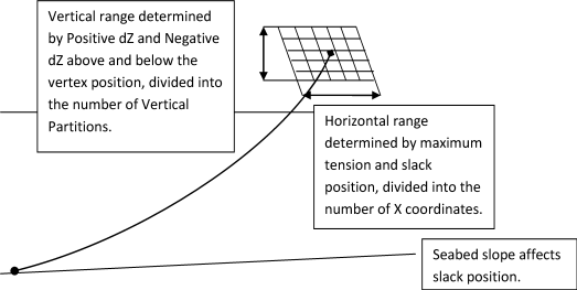
For cables attached between a fixed point and a structure (Connectivity set to ), the range of the possible end points of the cable is determined by Negative dZ Range of Expected Connection Point Vertical Motion (measured from the lowest anticipated database point to the connection point in the definition position) and Positive dZ Range of Expected Connection Point Vertical Motion (measured from the connection point in the definition position to the highest anticipated database point) along with the slack and maximum tension positions (including the effects of the global or cable-specific seabed slope). This area is then divided up to form a database of cable end positions and corresponding tensions which is used in the analysis. It is recommended that the full size of this grid is used, of 600 points, which is formed by the multiplication of Number of Vertical Partitions and Number of X Coordinates.
For cables attached between two structures (Connectivity set to ), where the Seabed Touchdown Expected option is set to No, the range of the possible end points of the cable is determined by the relative positions of the two structures along with the slack and maximum tension range. The cable is considered to be submerged in water of infinite depth. It is recommended that the full size of the database is used, of 600 points, which is formed by the multiplication of Number of Vertical Partitions and Number of X Coordinates.
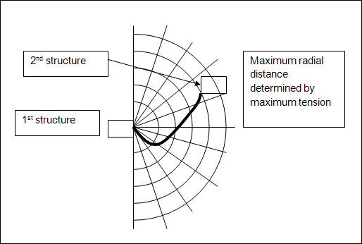
For cables attached between two structures where the Seabed Touchdown Expected option is set to No, the database uses a radial coordinate system in which Number of X Coordinates becomes the number of radial distances and the Number of Vertical Partitions is the number of angular positions.
For cables attached between two structures (Connectivity set to Structure to Structure), where the Seabed Touchdown Expected option is set to Yes, the range of the possible end points at either end of the cable is determined by Negative dZ Range of Expected Connection Point Vertical Motion (measured from the lowest anticipated database point to the connection point in the definition position) and Positive dZ Range of Expected Connection Point Vertical Motion (measured from the connection point in the definition position to the highest anticipated database point). If Global Sloped Seabed is non-zero, you must also specify the Maximum Radius of Start Connection Point Horizontal Motion (measured from the connection point in the definition position to the furthest anticipated database point). It is recommended that the full size of the database is used (600 points) which is formed by multiplication of Number of Vertical Partitions and Number of X Coordinates.
Caution: Generation of the database required for a Structure to Structure cable with Seabed Touchdown Expected may increase the computational cost and memory requirement of the analysis significantly. This option should be set to Yes only where there is any chance a cable will touch down.
Note: For a Structure to Structure cable which is resting on the seabed, the cable position illustrated in the Graphics panel will only account for the seabed effect after a Solve has been performed. For example, in a Stability Analysis, the cable may initially be shown hanging below the level of the seabed, but this is updated once the analysis has been solved.
Tip: Where the Global Seabed Slope is non-zero, it is recommended that the cable Start Connection Point is positioned on the structure with the smaller expected range of motion of the two connected structures. Minimizing the Maximum Radius of Start Connection Point Horizontal Motion will improve the accuracy of the generated database.
For more information on the different quasi-static databases generated for each cable configuration, see The COMP/ECAT/SSCB Data Records - Composite Catenary Mooring Line in the Aqwa Reference Manual.