


System Coupling provides you with the ability to execute a coupled analysis using High-Performance Computing (HPC) resources in parallel. You can run the analysis on a single machine or distributed on two or more machines. Distributed runs are executed directly or indirectly with a queuing system, with Linux support for LSF, PBS Pro, UGE, and SLURM.
Note: In the sections that follow, "machine" denotes a compute resource with multiple cores and a fixed amount of memory.
System Coupling always runs in parallel on two cores and has additional parallel execution features that work in conjunction with the automatic start-up of two or more participants. Load balancing of HPC resources is controlled via selecting the number of cores to be allocated to each participant and the algorithm for partitioning them. When participants are run in parallel along with System Coupling, it accelerates the heavyweight work performed during the simulation.
Note: When running a large case via HPC, you can free up resources by disabling the
creation of an initial snapshot. To do so, set the OutputControl.WriteInitialSnapshot to False.
For more information, see:
Set up your analysis, as described in Preparing for a Coupled Analysis.
To use parallel-specific command-line options when starting System Coupling, see Parallel Options for System Coupling.
Set up your coupled analysis.
Edit your data model settings.
To run an individual participant product in parallel mode, specify the participant's command-line execution details. For more information, see Parallel Options for Participant Products.
To run all coupling participants in parallel, specify how the participants are partitioned across compute resources. For more information, see Parallel Processing for Coupling Participants.
Run the solution.
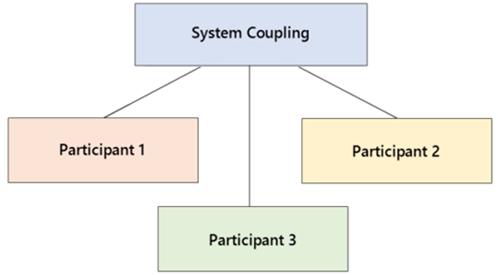
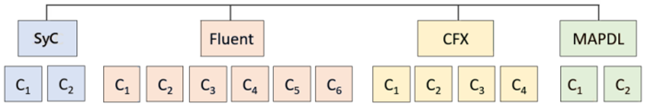
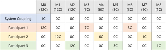
Parallel processing for co-simulation tends to be more involved than it is for single-solver simulations. A co-simulation involves, at minimum, three participants (that is, System Coupling and at least two coupling participants). Figure 12: Co-simulation with four coupling participants shows a co-simulation with four participants, each with different number of compute processes per participant. System Coupling provides participant partitioning capabilities, partitioning the simulation work across participants then allocating that work across available computing resources.
When setting up participants for parallel execution, you can set the following parameters to control the behavior of the run:
Machine List: The list of machines to be used and, where applicable, the number of cores each has available for the parallel run. For more information, see Machine List and Core Counts.
Participant Fractions: The fractions specifying the core count or fraction of compute resources to be allocated to each participant. For more information, see Resource Allocation Fractions.
Partitioning Algorithm: The algorithm used to specify the resource allocation method (machines or cores) and parallel execution mode (local or distributed) to be used. For more information, see Partitioning Algorithms.
The parallel execution details that were specified most recently — regardless of by what method — replace existing parallel values.
For more information, see:
System Coupling allows you to specify the list of machines to be used and, where applicable, the number of cores available on each machine for a parallel run.
In many cases, you will not specify the machine list and core counts for a parallel run. For example, when the machine list and core count are handled by a load manager or job scheduler, you do not need to specify them.
However, if you do want to explicitly specify or review the machine list and available cores, you can use the command-line options described in the Coupling Participant Parallel Options section of the System Coupling Settings and Commands Reference manual.
- When starting System Coupling (recommended):
Use the command-line options described in the Coupling Participant Parallel Options section of the System Coupling Settings and Commands Reference manual.
- When running the System Coupling GUI:
Open the Parallel solve setup dialog (accessed by right-clicking Outline | Setup | Coupling Participant) and:
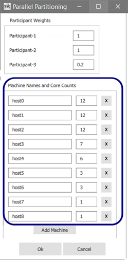
For Linux, add details under Machine Names and Core Counts.
For Windows, review auto-populated details under Local Machine Core Counts.
- When running the System Coupling CLI or defining custom participant partitioning:
Run the PartitionParticipants() command, using the MachineList argument to specify machine name and core count details.
For more information, see Participant Partitioning Examples.
When applying partitioning to coupling participants, you can use the ParallelFraction parameter to specify the core count or fraction of compute resources to be allocated to each participant. With regard to this setting, partitioning behavior depends on the parameter value and whether the default SharedAllocateMachines partitioning algorithm is used, as shown in the tables below.
In some cases, the resource allocation fractions provided by the default algorithm may not be optimal, depending on the participants involved and the co-simulation resource needs. For instance, the Mechanical APDL structural solver might run more optimally on a lower core count than the Fluent solver, so you might want to set a lower fraction for MAPDL.
Note: Resource allocation fractions are not supported for the
Custom participant
partitioning algorithm.
Table 22: Behavior when the ParallelFraction parameter is omitted and fractions are not provided
| Partitioning algorithm | Behavior |
|---|---|
|
SharedAllocateMachines |
Each participant will run on all the allocated cores. |
|
SharedAllocateCores DistributedAllocateMachines DistributedAllocateCores |
Each participant will run on an equal fraction of the total core count. |
Table 23: Behavior when the ParallelFraction parameter is used and fractions are provided
| Partitioning algorithm | Behavior |
|---|---|
|
SharedAllocateMachines |
If all the fractions are between Otherwise, all fractions are normalized with respect to the largest fraction. |
|
SharedAllocateCores DistributedAllocateMachines DistributedAllocateCores |
All fractions are normalized with respect to the sum of the fractions. |
System Coupling's algorithms provide for different permutations of parallel execution and resource allocation. By selecting an algorithm, you can control the parallel execution method (shared or distributed) and determine how participant work is allocated across compute resources (machines and cores).
When selecting a participant-partitioning algorithm, you specify the following information:
Resource allocation method: Determines whether available compute resources will be allocated as machines or cores.
Parallel execution mode: Determines whether participants will be run in shared parallel or distributed parallel (which are different than the local parallel and distributed parallel modes used for an individual participant). The table below compares the characteristics of each mode.
Table 24: Shared Parallel vs. Distributed Parallel execution modes
| Characteristics | Shared Parallel | Distributed Parallel1 |
|---|---|---|
|
Resource sharing |
Discrete participants share allocated machine resources. |
Discrete participants are executed on non-overlapping machines so that they do not share machine resources. |
|
Memory requirements |
Ideally, the number of processes run on the machine should not exceed the total core count on a machine. |
Useful when the co-simulation total memory requirements are greater than what is available for a shared simulation (that is, if the required memory to run in shared mode exceeds a machine's total memory). |
|
Resource requirements |
Multiple machines may be utilized, and the total number of required machines is dictated by the participant requiring the most resources. |
Depending on how the cores are allocated, participants may end up sharing resources on some machines. The number of machines with shared resources may be as high as the total number of participants. |
| 1: Distributed Parallel execution is supported only for Linux systems. | ||
For more information, see:
When choosing a participant partitioning algorithm, consider the resources needed for each participant, the number of machines/cores that are available, and how those resources might be allocated to best meet your parallel-processing requirements.
The following algorithms are available:
SharedAllocateMachines: Participants share both machines and cores. (default value)
Note: When this algorithm is used and simultaneous solutions are enabled, partitioning behavior changes slightly. For more information, see Execution of Simultaneous Participant Solutions.
SharedAllocateCores: Participants share machines but not cores.
DistributedAllocateCores: Participants minimally share cores and machines. (Linux only)
DistributedAllocateMachines: Participants never share cores or machines. (Linux only)
Custom: Participants use machines and cores as specified in the custom partitioning information you provide via the PartitionParticipants() command's PartitioningInfo argument.
For many co-simulations, the default
SharedAllocateMachines algorithm is often the best
choice. It behaves similarly to the methods used by individual solvers,
providing for full utilization of all the allocated cores, and generally
results in the best overall performance and scaling.
The other three "allocate" algorithms are provided as means of handling situations for which the default algorithm is not appropriate. For instance, if the total memory available on a machine is insufficient to handle running more than one participant, then you can use the non-default algorithm that best fits your parallel setup.
The Custom algorithm allows you to partition
participants in a specialized way not offered by the other
algorithms.
The tables below summarize the advantages and disadvantages generally associated with each of System Coupling's participant partitioning algorithms.
| SharedAllocateMachines | |
|---|---|
| Pro: |
Allows for full utilization of all cores (no idle cores) |
| Cons: |
Machines must have enough memory for all participants (highest memory demand) |
| SharedAllocateCores | |
|---|---|
| Pro: |
Cores are more evenly loaded – a better option for low memory machines |
| Cons: |
Cores remain idle when individual participants are executing |
|
Participants must be tolerant of distributed memory execution | |
|
The last participant may run on more machines if high core count machines are consumed by the other participants | |
| DistributedAllocateMachines (Linux only) | |
|---|---|
| Pros: |
Participants have complete access to all machine resources |
|
Useful if solving with participants that have high memory use | |
|
Shared memory parallel gets higher utilization (better scaling for a participant) | |
| Cons: |
Cannot control the number of cores to be assigned to each participant |
|
Last participant may get fewer cores | |
|
Only useful if requesting that resources are allocated exclusively, so you know the number of cores on each machine | |
| DistributedAllocateCores (Linux only) | |
|---|---|
| Pros: |
Participants have complete access to all machine resources |
|
Useful if solving with participants that have high memory use | |
|
Useful if you are requesting that resources are allocated exclusively | |
|
Shared memory parallel gets higher utilization (better scaling for a participant) | |
| Cons: |
Cores remain idle when individual participants are executing |
|
You may get overlap (sharing) but the maximum is equal to the total participant count | |
|
The last participant may run on more machines if high core count machines are consumed by the other participants | |
| Custom | |
|---|---|
| Pros: |
Useful if you need to partition participants in a way that is not possible using other algorithms |
|
Allows user to control the number of cores assigned to each participant | |
| Cons: |
Requires user intervention to manually query and assign machines and cores |
This section provides a description and usage example for each of System Coupling's participant partitioning algorithms.
Note that all the examples share the following setup details:
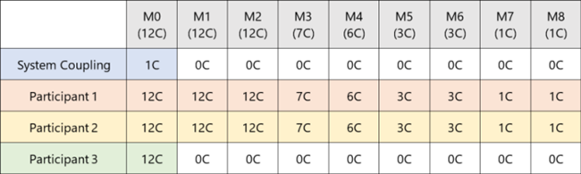
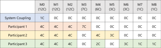
There are 57 cores with the same uneven distribution across nine machines, which are designated as M0 through M8.
System Coupling runs on the first machine on a single core.
Each example assumes that the machine list has already been set up using one of the methods shown below.
The figures below show the three methods you can use to set up the machine list and core count for the examples that follow:
Example 26: Machine list and core counts specified using the --cnf command-line option (Linux only)
> "$AWP_ROOT242/SystemCoupling/bin/systemcoupling" --cnf="host0:12,host1:12,host2:12,host3:7,
host4:6,host5:3,host6:3,host7:1,host8:1"  -R run.py
Example 27: Core counts specified using the -t command-line option
The specified core count cannot exceed the number of cores available on the local machine.
"%AWP_ROOT242%\SystemCoupling\bin\system coupling.bat" -t6 -R run.py
Example 30: Machine list and core counts specified using the PartitionParticipants() command (Linux)
> PartitionParticipants(MachineList = [
	{'machine-name' : 'host1', 'core-count' : 12},
	{'machine-name' : 'host2', 'core-count' : 12},
	{'machine-name' : 'host3', 'core-count' : 12},
	{'machine-name' : 'host4', 'core-count' : 7},
	{'machine-name' : 'host5', 'core-count' : 6},
	{'machine-name' : 'host6', 'core-count' : 3},
	{'machine-name' : 'host7', 'core-count' : 3},
	{'machine-name' : 'host8', 'core-count' : 1},
	{'machine-name' : 'host9', 'core-count' : 1}
	])
Example 31: Machine list and core counts specified using the PartitionParticipants() command (Windows)
In this case, you must specify the name of the local machine, which can be found using the Python socket module, and then specify the core count.
import socket

    PartitionParticipants(MachineList = [{'machine-name' : socket.gethostname(),
    'core-count' : 12}])
Note: Because all the partitioning examples that follow use the same machine/core setup, the machine list and core counts are the same for all of them. Only the partitioning algorithms and resource allocation fractions change for each example.
Participants share both machines and cores.
In the examples below, Participant-1, Participant-2, and Participant-3 have been allotted fractions of 1, 1, and 1/5, respectively.
Example 32: GUI setup for the default Shared Allocate Machines algorithm with machines allocated by fractions (Linux only)
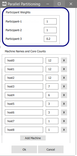
Note: A Windows GUI example is not shown because distributed parallel is not supported on Windows. The dialog's machine name and core counts fields are auto-populated from the local host and cannot be edited.
Example 33: Data model setup for the SharedAllocateMachines algorithm with machines allocated by fractions
dm = DatamodelRoot()

dm.AnalysisControl.PartitioningAlgorithm = 'SharedAllocateMachines'
dm.CouplingParticipant['PARTICIPANT-1'].ExecutionControl.ParallelFraction = 1.0
dm.CouplingParticipant['PARTICIPANT-2'].ExecutionControl.ParallelFraction = 1.0
dm.CouplingParticipant['PARTICIPANT-3'].ExecutionControl.ParallelFraction = 1.0/5.0
Example 34: PartitionParticipants() setup for the SharedAllocateMachines algorithm with machines allocated by fractions
PartitionParticipants(AlgorithmName = 'SharedAllocateMachines',
        NamesAndFractions = [('PARTICIPANT-1', 1.0),
                            ('PARTICIPANT-2', 1.0),
                            ('PARTICIPANT-3', 1.0/5.0)])
Participants share machines but not cores.
The machines are sorted by core count and allocated in blocks, which are sized by the number of participants. This helps to ensure that each participant gets cores on machines with highest total core counts, keeping any inter-process communication local to a machine.
In the examples below, Participant-1, Participant-2, and Participant-3 have each been allotted 19 cores.
Example 36: Data model setup for the SharedAllocateCores algorithm with even allocation of cores
DatamodelRoot().AnalysisControl.PartitioningAlgorithm = 'SharedAllocateCores'
Example 37: PartitionParticipants() setup for the SharedAllocateCores algorithm with even allocation of cores
Participants minimally share cores and machines. Available for Linux.
The machines are sorted by core count and allocated into blocks, which are sized by the number of participants. This helps to ensure that each participant gets cores on machines with highest total core counts, keeping any inter-process communication local to a machine.
In the examples below, Participant-1, Participant-2, and Participant-3 have each been allotted 19 cores.
Example 38: Data model setup for the DistributedAllocateCores algorithm with even allocation of cores
DatamodelRoot().AnalysisControl.PartitioningAlgorithm = 'DistributedAllocateCores'
Example 39: PartitionParticipants() setup for the DistributedAllocateCores algorithm with even allocation of cores
PartitionParticipants(AlgorithmName = 'DistributedAllocateCores')
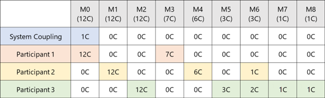
Participants never share cores or machines. Available for Linux.
The machines are sorted by core count and allocated in blocks, which are sized by the number of participants. This helps ensure that each participant gets cores on machines with highest total core counts, keeping any inter-process communication local to a machine.
In the examples below, Participant-1, Participant-2, and Participant-3 have each been allotted 3 machines.
Example 41: Data model setup for the DistributedAllocateMachines algorithm with even allocation of cores
DatamodelRoot().AnalysisControl.PartitioningAlgorithm = 'DistributedAllocateMachines'
Example 42: PartitionParticipants() setup for the DistributedAllocateMachines algorithm with even allocation of cores
PartitionParticipants(AlgorithmName = 'DistributedAllocateMachines')
Based on how available machines are assigned, the Custom algorithm allows you to
configure machines to run either in shared parallel or distributed
parallel, even within the same coupled analysis. It also allows for
participant partitioning to be applied selectively, so that some
participants run as specified by the algorithm while others run in their
default mode.
In each of the examples that follow, it is assumed that each machine list includes multiple machines.
Example 44: Editing the data model to configure distributed participant execution
In this example, there are two participants and two machine lists.
Both participants are running in distributed parallel. Each participant is distributed across the machines in the list assigned to it.
machineList1 = [
    {'machine-name' : 'machine-1', 'core-count' : 5},
    {'machine-name' : 'machine-2', 'core-count' : 7}]
machineList2 = [
    {'machine-name' : 'machine-1', 'core-count' : 3},
    {'machine-name' : 'machine-3', 'core-count' : 7}]
partitioningInfo = {'MAPDL' : machineList1, 'CFX-2' : machineList2}

PartitionParticipants(PartitioningInfo = partitioningInfo)
Example 45: Editing the data model to configure distributed, shared, and serial participant execution
In this example, there are five participants and two machine lists.
The MAPDL participant runs distributed parallel across the machines in machineList1.
The CFX participants run in shared parallel across the machines in machineList2.
The remaining two participants are not included in the partitioning information. Partitioning is not applied, and participants run using their default settings.
partitioningInfo = {
    'MAPDL-1' : 'machineList1',
    'CFX-2' : 'machineList2',
    'CFX-3' : 'machineList2'}
Partitioning coupling participants allows you to control how they are distributed across compute resources, specifying the partitioning algorithm to be applied, how available resources will be allocated, and what machines will be available for the parallel execution.
To apply partitioning to coupling participants, your coupled analysis must meet the following prerequisites:
System Coupling has been started with one or more cores.
At least one participant is defined.
No participants are already started.
Note: When simultaneous execution of participant solutions is enabled, the explicit application of partitioning is changed as described in Partitioning Algorithms.
For more information, see:
You may apply partitioning using the System Coupling GUI.
Note: If you plan to use the Custom algorithm, use the steps
outlined in Applying Custom Participant Partitioning.
Specify the partitioning algorithm.
In the Outline tree under Setup, select Analysis Control.
Related settings are shown under Properties.
Set Partitioning Algorithm to the algorithm to be applied to the analysis.
For information on available algorithms, see Partitioning Algorithms.
Specify the resource allocation fractions for each participant.
In the Outline tree under Setup, right-click Coupling Participant and select Parallel solve setup.
The Parallel Partitioning dialog opens.
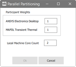
Under Participant Weights, specify the resource weighting for each coupling participant as a real number.
For more information, see Resource Allocation Fractions.
Specify and/or verify the available machines and cores.
The method by which machines and core counts are specified is determined by the platform being used, as follows:
Windows:
The fields under Local Machine Core Count are auto-populated with the name of the local machine (localhost) and the number of cores available on that machine.
Note: Because distributed parallel processing is not supported for Windows, specification of a machine and cores is not available here. However, you can use the -t command-line argument when starting System Coupling to specify core counts.
Linux:
Under Machine Names and Core Counts, specify the name of each machine and the number of cores available on that machine.
Click Add Machine to add machines and their core counts to the list.
For details on this and other methods of setting this information, see Machine List and Core Counts.
Close the dialog, as follows:
For Windows, click .
For Linux, click .
When using System Coupling's CLI, apply partitioning to coupling participants using a combination of command-line arguments and data model edits.
Note: If you plan to use the Custom algorithm, use the steps
outlined in Applying Custom Participant Partitioning.
Specify the number of cores to be used by the local machine.
When starting System Coupling, use the -t command-line argument to specify the number of cores to be used when running on the local machine.
> "%AWP_ROOT242%\SystemCoupling\bin\systemcoupling" -t4 -R run.py
Tip: On a Linux system, you can explicitly set the machine list and the number of cores to be used by each machine. To do so, issue the --cnf command-line argument when starting System Coupling. However, if a Linux job is being submitted to a job scheduler (that is, PBS, LSF, SLURM or UGE), then the machine list is automatically detected from the scheduler environment if you do not provide it via the command-line arguments (for example, -t, --cnf) or the PartitionParticipants() command.
For more information, see Machine List and Core Counts.
For information on the -t and --cnf arguments, see Coupling Participant Parallel Options in the System Coupling Settings and Commands Reference manual.
Specify the partitioning algorithm.
To specify the partitioning algorithm to be applied to the coupled analysis, edit the AnalysisControl.PartitioningAlgorithm setting in the data model.
DatamodelRoot().AnalysisControl.PartitioningAlgorithm = 'DistributedAllocateCores'
For information on available algorithms, see Partitioning Algorithms.
Note:Distributed parallel processing is not supported for Windows systems.
When running either shared or distributed execution modes, CFX and Fluent participants should be the last participants added to the analysis because they tolerate distributed parallel processing well.
Specify the resource allocation fractions for each participant.
To specify the core count or fraction of compute resources to be allocated to each participant, edit each participant's ExecutionControl.ParallelFraction setting in the data model.
DatamodelRoot().CouplingParticipant['FLUENT-2'].ExecutionControl.ParallelFraction=1.0/5.0
For more information, see Resource Allocation Fractions.
Note: The PartitionParticipants() command is available as an alternative method of applying partitioning to coupling participants.
If you need to partition participants in a specialized way that is not
offered by System Coupling's system-defined partitioning algorithms, you can
use the Custom
partitioning algorithm, which allows you to assign machines to
participants as needed.
Note: Resource allocation fractions are not used for custom participant partitioning.
To use custom partitioning, review the following sections:
When you run the PartitionParticipants() command, the PartitioningInfo argument accepts a dictionary specifying what machine resources are assigned to each participant. Each tuple pair in the dictionary consists of:
a participant name as key
a machine list (a list of dictionaries specifying available machines and their core counts) as value
When you set partitioning details using the PartitioningInfo argument, System Coupling uses the Custom partitioning algorithm automatically and blocks all other partitioning algorithms.
Note: This means that if you attempt to use any other PartitionParticipants() argument in conjunction with the PartitioningInfo argument, you will receive an error.
If you provide incomplete information for the PartitioningInfo argument — that is, when either the name of an existing participant is not included or an included participant is associated with an empty machine list — then the affected participant executes using its default parallel settings.
To get values for the PartitioningInfo argument, obtain lists of available participants and machines.
To get participants, query the CouplingParticipant object.
>>> DatamodelRoot().CouplingParticipant.GetChildNames()

['MAPDL-1', 'FLUENT-2', 'FLLUENT-3']
To get machines, run the GetMachines() command.
>>> GetMachines()

[{'machine-name' : 'machine-1', 'core-count' : 4}, {'machine-name' : 'machine-2',
'core-count' : 8}, {'machine-name' : 'machine-3', 'core-count' : 12}]
You may either obtain these lists as shown above or include the queries in a Python script, as shown in Applying Custom Partitioning by Running a Script.
To apply custom partitioning, run the PartitionParticipants() command, using the PartitioningInfo argument to specify participants and the machines assigned to them.
Note:
When you specify partitioning details using the PartitioningInfo argument, the
Customalgorithm is used automatically.If AlgorithmName has been set to
Custommanually (not recommended), then you must still set using the PartitionParticipants() command's PartitioningInfo argument.
In the example below, each of the three participants has one machine assigned to it. In this case, the AlgorithmName argument is not required because partitioning details are set by the PartitioningInfo argument.
>>>PartitionParticipants(
      PartitioningInfo = {
          'MAPDL-1': [{'machine-name' : 'machine-1', 'core-count' : 4}],
          'CFX-2': [{'machine-name' : 'machine-2', 'core-count' : 4}]
      }
    )
To apply custom partitioning in the GUI, specify partitioning parameters by running the PartitionParticipants() command in the Command Console. For details, see Applying Custom Partitioning by Running a Command.
When the command is executed, the Algorithm Name property is set to Custom automatically and other partitioning algorithms are blocked.
You can apply custom partitioning by running a script in System Coupling's CLI.
allMachines = GetMachines()

# all AEDT participants go on the first core
aedtMachines = []
aedtMachines.append({'machine-name' : allMachines[0]['machine-name'], 'core-count' : 1})

# all FLUENT participants go on the rest of the cores
fluentMachines = []
fluentMachines.append(allMachines[1])
fluentMachines.append({'machine-name' : allMachines[0]['machine-name'], 'core-count' :
    allMachines[0]['core-count'] - 1})

partitioningInfo = {}

 for participant in DatamodelRoot().CouplingParticipant.GetChildren():
    participantName = participant.GetName()
    if participant.ParticipantType == "AEDT":
        partitioningInfo[participantName] = aedtMachines
    else if participant.ParticipantType == "FLUENT":
        partitioningInfo[participantName] = fluentMachines

PartitionParticipants(PartitioningInfo = partitioningInfo)
When running in parallel, System Coupling always runs on two cores. For information on parallel command-line options, see System Coupling Parallel Options in the System Coupling Settings and Commands Reference manual.
If you also plan to use parallel processing for the coupling participants, then you may wish to review Coupling Participant Parallel Options.
Coupling participant setup files do not include parallel processing information. To run an individual coupling participant product in parallel execution mode, you must introduce solver-specific parallel details using settings defined under the participant's ExecutionControl singleton.
When parallel customizations for an individual participant are needed, you may use these execution control settings instead of the partitioning functionality described in Parallel Processing for Coupling Participants.
When System Coupling starts the coupled analysis execution, these arguments are picked up from the data model and used to start the participant solver. If the specified arguments conflict with default values set by System Coupling, the new values override the System Coupling defaults.
For more information, see:
All coupling participants have an AdditionalArguments execution control setting. You may use this setting to enter arguments defining parallel details for the participant.
Note: Some participants populate this setting with default values. For details, see the participant's product documentation.
You may add solver-specific arguments either in the GUI or the CLI.
- Adding solver-specific parallel arguments in the GUI
When using the System Coupling GUI, specify solver-specific parallel arguments by adding them to the Additional Arguments setting, as follows:
In the Outline tree under Coupling Participant, locate and expand the branch for the participant object.
Under the participant object, click Execution Control.
The participant's execution controls are shown in the Properties pane.
Enter the solver-specific arguments into the Additional Arguments field.
- Adding solver-specific parallel arguments in the CLI
When using the System Coupling CLI, specify solver-specific parallel arguments by adding them to the AdditionalArguments setting in the participant's execution controls, as shown in the example below:
Example 46: Adding CFX parallel arguments from the CLI on Windows
DatamodelRoot().CouplingParticipant['FLUENT-2'].ExecutionControl.AdditionalArguments
= cfx5solve -def model.def -par-dist 'hosta,hostb*2,hostc*4'
For AEDT coupling participants, additional parallel processing settings are defined under the participant's ExecutionControl singleton. Each setting corresponds to functionality available in Maxwell's Analysis Configuration dialog and as command-line arguments for HPC integration.
You can use these settings to configure Maxwell to use automatic or manual HPC distribution. For more information, see:
System Coupling supports the use of auto-distribution, a Maxwell solver setting that
allows Maxwell to estimate optimal HPC usage for each Maxwell solver
type. To use auto-distribution in a System Coupling analysis, set the
AutoDistributionSettings execution control to
True.
Auto-distribution is an evolving capability that performs well in many circumstances, as follows:
For Maxwell 2D Transient simulations, the automatic setting generally makes very effective usage of the Time Decomposition Method (TDM, or the
Transient
								Solver
HPC distribution type).For Maxwell 3D Transient simulations, the automatic setting attempts to use the Time Decomposition Method with an estimate and limits for memory usage. However, memory usage exceeding the system limits will result in a crash. In this case, you will need to use manual HPC distribution settings (see below).
For Maxwell 3D Eddy Current simulations, the automatic setting uses shared-memory HPC by default. To use multiple nodes, you will need to manually set the distribution type to Solution Matrix.
You may enable auto-distribution in System Coupling's GUI or CLI.
- Enabling Auto-Distribution in the GUI
Select the AEDT participant's Execution Control branch.
In the Properties pane, set Auto Distribution Settings to
True.
- Enabling Auto-Distribution in the CLI
Set AutoDistributionSettings to
True, ensuring that you use the internal participant object name assigned by System Coupling.DatamodelRoot().CouplingParticipant['AEDT-1']. ExecutionControl.AutoDistributionSettings = True
When auto-distribution is enabled, the task count is set to -1 and the machine list is formatted as
follows: list=machineA:-1:<nCoresA>,
machineB:-1:<nCoresB>,…
Tip: This setting corresponds to Maxwell Use Automatic Settings check box and -auto command-line argument (shown below).
-distributed -auto -machinelist list=hostA:-1:32,hostB:-1:24,hostC:-1:48
To edit Maxwell's distribution settings manually, set System Coupling's
AutoDistributionSettings parameter to
False. This allows
you to control the HPC distribution types and specify how many cores
per task will be used to distribute the HPC solution.
Note: Distributed parallel execution is not supported when auto-distribution
is disabled. That is, when AutoDistributionSettings
is set to False,
only one machine may be specified by the
-machinelist argument.
When auto-distribution is disabled, the following parallel settings are available.
- IncludeHPCDistributionTypes
Required. Enter a string list of the distribution type(s) to be included for a distributed run. Available distribution types are
Solution MatrixandTransient Solver. Empty by default.Tip: This setting corresponds to Maxwell's Job Distribution tab and -includetypes argument (shown below).
-distributed "include types=Solution Matrix, Transient Solver" -machinelist list=hostA:32:32- NumberOfCoresPerTask
Enter an integer greater than or equal to one to indicate the number of parallel cores to be used per task. Default value is
1.Any cores per task will be used as a shared-memory HPC speed-up (multi-threading) for each task. The number of tasks is determined as follows:
nTasks = floor(nCores /
									nCoresPerTask)
By default, the number of tasks is equal to the number of cores. For example:
If a machine has a core count of
32and NumberOfCoresPerTask is set to1, then there will be32tasks.If NumberOfCoresPerTask is changed to
2, then there are16tasks.If NumberOfCoresPerTask is changed to
3, then the floor function is applied and there are10tasks.
Tip: This setting corresponds to the task count and core count for Maxwell's Machines tab and -machinelist argument (shown below).
-distributed "include types=Solution Matrix" -machinelist list=hostA:16:32
- BatchOptions
Enter a string to specify the specified batch option arguments to be applied to the run.
Note: When this option is used from the command line, the escape characters \" are required.
Tip: This setting corresponds to Maxwell's Options tab and -batchoptions argument (shown below).
-distributed "include types=Solution Matrix" -machinelist list=hostA:32:32
-batchoptions "\"'Maxwell 3D/NumCoresPerDistributedTask'=10\""
Example 47: Setting distribution settings manually from the command line
When editing distribution settings from the command line, make sure to use the internal participant object name assigned by System Coupling.
DatamodelRoot().CouplingParticipant['AEDT-1'].ExecutionControl.AutoDistributionSettings = False
DatamodelRoot().CouplingParticipant['AEDT-1'].ExecutionControl.IncludeHPCDistributionTypes = ['Transient Solver', 'Solution Matrix']
DatamodelRoot().CouplingParticipant['AEDT-1'].ExecutionControl.NumberOfCoresPerTask = 2
DatamodelRoot().CouplingParticipant['AEDT-1'].ExecutionControl.BatchOptions = "\"'Maxwell 3D/NumCoresPerDistributedTask'=10\""