After System Coupling has associated source and target locations, it generates data on the mapped target location, and when applicable, the unmapped target locations.
When data is transferred to the target location, its fidelity is limited by the least-resolved side of the interface. For example, if the target mesh is significantly coarser than the source mesh, then fine-scale features of the source solution may be missed in mapping. Similarly, if the target mesh is significantly finer than the source mesh, then the target data may exhibit pathologies due to the coarseness of the source mesh (that is, piece-wise constant or linear variation of source data may be apparent over groups of elements on the target side).
For information on the methods used to data on target locations, see:
System Coupling calculates mapping weights and then uses the weights to interpolate the source data onto the target.
The algorithm System Coupling uses is determined by the type of mapping being performed plus the topologies of involved participant regions. Available data-generation algorithms are listed below.
Profile-Preserving Mapping
- Shape Functions
For profile-preserving mapping from surface source mesh regions to surface target mesh regions, mapping weights are generated using shape functions.
Note: System Coupling's interpolation is always at least as accurate as the interpolation used by the source participant solver. For details, see the relevant participant product documentation.
- Radial Basis Functions
For profile-preserving mapping from volume regions to volume regions, mapping weights are generated using radial basis functions.
For volume-to-volume mapping with source data on elements, an element-based RBF algorithm maps the data to overlapping locations.
- Element-Weighted Averages
For profile-preserving mapping from volume mesh regions to 2D surface mesh regions, weights are generated using an element-weighted average.
Conservative Mapping
- Intersection
For conservative mapping with any combination of topologies, mapping weights are generated by intersecting the source and target mesh elements, followed by transferring of the data from source to target, based on the extent to which the source and target elements are overlapping.
System Coupling handles the lack of associated source data according to the type of mapping being performed plus the topologies of involved participant regions.
Note: The concept of "non-overlapping" locations is not applicable for point clouds.
- Conservative Mapping
Non-overlapping target elements are assigned a value of zero.
- Profile-Preserving Mapping
Target data is generated on non-overlapping target locations based on the values of other mapped locations. The method used is determined by the topology of the target region, as follows:
Copy or extrapolate target values from overlapping locations on the target side (depending on the value of the UnmappedValueOption setting)
This method is used when the source and target both consist of surface mesh regions.
Copy the value from the nearest source-side location
This method is used for all other mapping algorithms.
The table below shows the different association and target data generation algorithms for profile-preserving and conservative mapping between regions with different topology/region discretization type combinations.
| Mapping Type | Topology | Region Discretization Type | Target Data Generation | |||
|---|---|---|---|---|---|---|
| Source | Target | Source | Target | On Overlapping Locations (Mapping Weights) | On Non-Overlapping Locations | |
| Profile-Preserving |
Volume |
Surface |
Mesh |
Mesh |
Element-Weighted Averages |
Calculated from Overlapping Target Locations1 |
|
Surface |
Surface |
Mesh |
Mesh |
Shape Functions |
Calculated from Overlapping Target Locations1 | |
|
Point Cloud |
Point Cloud |
Radial Basis Functions |
N/A | |||
| Point Cloud | Mesh | Radial Basis Functions | N/A | |||
| Mesh | Point Cloud | Shape Functions | N/A | |||
|
Volume |
Volume |
Mesh2 |
Mesh |
Radial Basis Functions |
Nearest Source Point Value3 | |
|
Point Cloud |
Point Cloud |
Radial Basis Functions |
N/A | |||
|
Mesh |
Point Cloud |
Radial Basis Functions |
Nearest Source Point Value3 | |||
| Point Cloud | Mesh | Radial Basis Functions |
Nearest Source Point Value3 | |||
| Conservative |
Surface |
Volume |
Mesh |
Mesh |
Intersection |
Zero value |
|
Surface |
Surface |
Mesh |
Mesh |
Intersection |
Zero value | |
|
Volume |
Volume |
Mesh |
Mesh |
Intersection |
Zero value | |
|
1: For profile-preserving mapping onto a target surface, target values can be either copied or extrapolated from the nearest target-side node, depending on the value of the UnmappedValueOption setting. 2: When source data are on element centroids and the element's neighborhood (surrounding elements that share a face with it), an element-based version of the Radial Basis Function algorithm is used. | ||||||
For data transfers of intensive variables, the following algorithms are used to generate data for mapped target locations:
For transfers of intensive variables between surfaces, Shape Functions are used to generate target data for mapped locations. The type of shape functions selected are determined by the source mesh provided by the coupling participant. System Coupling uses linear shape functions for source meshes with linear elements, and quadratic shape functions for source meshes with quadratic elements.
Quantities located on source mesh nodes are mapped to target mesh nodes, as shown in the figure below.
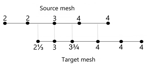
Mapping weights are generated using finite element shape functions of the source element associated with each target node, as shown in the figure below.
Figure 36: Mapping weights generated for a target node, based upon its projection onto a source element via Shape Function mapping
For transfers of intensive variables between volumes, Radial Basis Functions (RBF) are used to generate target data for overlapping target locations.
The location of the source data determines the RBF algorithm used to map data to overlapping target mesh locations (either element centroids, mesh nodes, or point cloud nodes), as illustrated in the diagrams below.
When source points are on mesh nodes:
A node-based RBF algorithm maps the data to overlapping target locations.
Non-overlapping target locations receive values from the nearest source point value.
When source points are on element centroids:
An element-based RBF algorithm maps the data to overlapping target locations.
Non-overlapping target locations receive values from the centroid of the intersecting element.
Generation of target data on non-overlapping locations is not applicable for point cloud-to-point cloud mapping.
For volumes, the element-based RBF algorithm, which performs mapping directly on the element centroids, is used by default. A beta setting allows you to revert to the node-based RBF algorithm, which reconstructs elemental data on element nodes and then performs mapping on the reconstructed data.
For surfaces, the element-based RBF algorithm is available as a beta feature.
Note: For details, see Activate System Coupling Hidden Features.
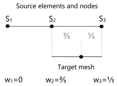
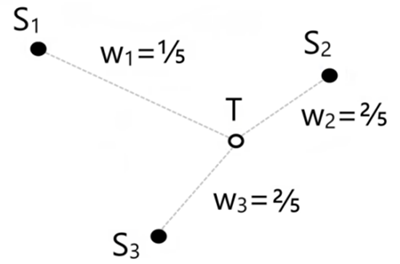
Mapping weights are generated using radial basis functions (RBFs) for the source nodes or centroids that define the associated source elements. Example weights are shown in the figure below.
Figure 38: Example mapping weights wi generated for a target node (T), based on the distance to nodes with the associated source elements Si via Radial Basis Function mapping
For transfers of intensive variables from a volume to a surface, Element-Weighted Averages are used to generate target data for mapped locations.
Quantities located on the source mesh nodes are mapped to target mesh nodes, as shown in the figure below.
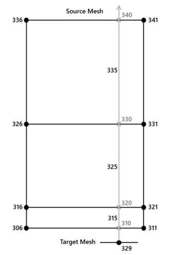
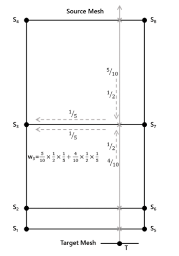
Intersection points are created by projecting the target (surface) nodes through the source (volume) elements. Mapping weights are generated by taking a length-weighted average of the line segment within each intersecting volume element. For an illustration, see the figure below.
Figure 40: Mapping weights generated for a target node (T), based upon its extrusion onto source elements via Element Weighted Average mapping. Representative weight calculation is shown for node 3; other weights are computed in a similar manner.
For data transfers of extensive variables, the Intersection algorithms are used to generate target data. There are two variations of this algorithm, and the variation used is determined by participant region topologies
This version of the Intersection algorithm is used when extensive variables are transferred between two surfaces or between two volumes.
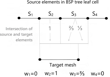
Data located on the source mesh elements are mapped to target mesh elements, as shown in the figure below.
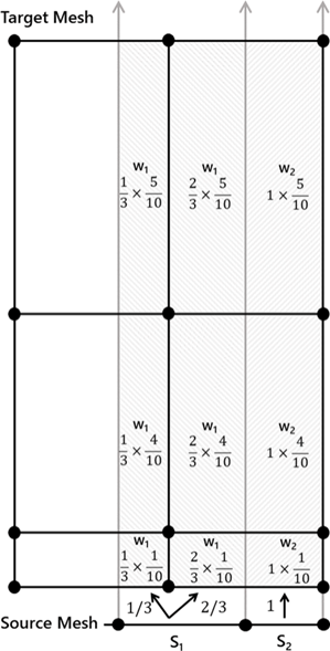
Mapping weights are generated based upon information extracted from intersecting the target element with the source elements. In particular, the size of each intersected region relative to the size of the respective source element is used, as shown in the figure below.
Figure 42: Mapping weights generated for a target element, based on its intersection with source elements between like topologies
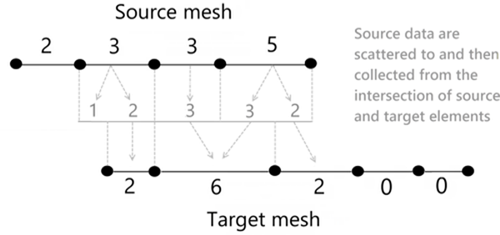
This version of the Intersection algorithm is used for unlike topologies (that is, applied when the Extrusion association method is used) is used when extensive variables are transferred from a surface to a volume.
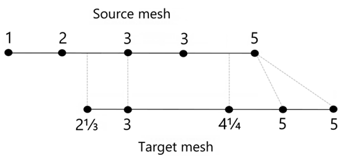
Data located on the source mesh elements are mapped to target mesh elements, as shown in the figure below.
Figure 43: Example input and output for conservative mapping for Intersection for surface-to-volume mapping. Circled values are the total for the elements.
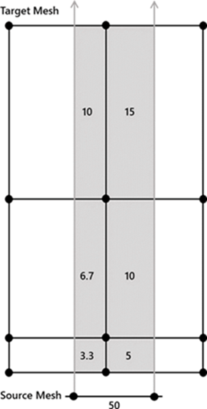
When the target (surface) elements are extruded onto source (volume) elements, intersections are created between the resulting target (pseudo-volumetric) elements and the source (volume) elements. Mapping weights are generated by taking a volume-weighted average of the intersecting volume between the target and source elements. For an illustration, see the figure below.
Figure 44: Mapping weights generated for a target node, based upon its extrusion onto a target element via the Intersection algorithm for surface-to-volume mapping