


To begin the mapping process, System Coupling creates associations between locations on the source mesh and locations on the target mesh, essentially placing them in the same simulation space. The association process begins with a Binary Space Partitioning (BSP) search to quickly identify the required set of candidate mesh locations to be used in the generation of mapping weights. For more information, see Binary Space Partitioning Algorithm.
When a source location overlaps a target location and an association is created, the target location is said to have been successfully "mapped." When no overlap exists and no association can be made, the target location is said to have been left "unmapped."
There are four methods used to associate source and target locations: Projection, Coincident, Extrusion, and Search Radius. The method used is determined by the topologies and region discretization type of the participant regions involved in the mapping, as follows:
- Projection
Used for surface-to-surface (2D-to-2D) mapping when the region discretization type is set to
Mesh Region.Mesh from one side of the interface is projected (or scattered) onto the other side of the interface, as follows:
For profile-preserving mapping, the target mesh is projected onto the source mesh. For an illustration, see Shape Functions.
For conservative mapping, the source mesh is projected onto the target mesh. For an illustration, see Intersection Algorithm for Surface-to-Surface and Volume-to-Volume Mapping .
- Coincident
Used for volume-to-volume (3D-to-3D) mapping when the region discretization type is set to
Mesh Region.Source mesh is mapped directly to the target locations.
For an illustration of profile-preserving mapping, see Radial Basis Functions.
For an illustration of conservative mapping, see Intersection Algorithm for Surface-to-Surface and Volume-to-Volume Mapping .
- Extrusion
Used for volume-to-surface (3D-to-2D) and surface-to-volume (2D-to-3D) mapping.
Source mesh is extruded onto the target mesh.
For an illustration of profile-preserving mapping, see Element-Weighted Averages.
For an illustration of conservative mapping, see Intersection Algorithm for Surface-to-Volume and Volume-to-Surface Mapping .
Note: In these cases, the surface must be within one diameter of the volume mesh for mapping to occur. For best results, ensure that the orientation of the surface and its location with respect to the volume are consistent with your problem setup.
- Search Radius
Used for point cloud-to-point cloud mapping.
Nearby source points are identified for each target location.
For an illustration of profile-preserving mapping, see Radial Basis Functions.
Conservative mapping is not defined in this case.
A Binary Space Partitioning (BSP) tree algorithm is used to quickly identify the required set of candidate mesh locations to use for generating mapping weights.
The BSP algorithm fits a uniform structured grid of two cells to the source region(s). Each cell that contains more than a predetermined number of source mesh locations is recursively subdivided into two new cells in a direction that is orthogonal to the preceding division. This continues to form a hierarchical tree structure, as shown in the figure below, until either the maximum number of levels in the hierarchy is reached or the predetermined number of source mesh locations per tree cell is reached. BSP tree cells at this level are referred to as "leaf cells."
Figure 34: Example of a BSP tree mesh on a 2D target domain, which extends naturally to 3D (source mesh locations not shown for clarity)
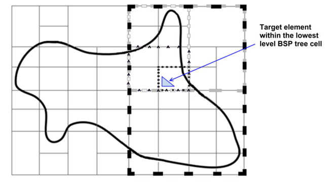
Each target mesh location is ultimately associated with one or more leaf cells. Efficiency is realized by associating the target mesh locations with a cell at each level within the tree hierarchy, starting with the highest (largest) cells first.
From here, the association process varies, as follows:
- Profile-Preserving Mapping
The association goes from target to source.
Once a target node is associated with a leaf cell(s), it is associated with the most suitable source element and/or nodes.
- Conservative Mapping
The association goes from source to target.
Once the source element is associated with a leaf cell(s):
For transfers to surface target regions, the source element is associated with intersecting target elements. Care is taken to appropriately consider the relative orientation and normal distance between associated source and target elements.
For transfers to volume target regions, the source element is associated with intersecting target elements.