10.3.2. Fitting Procedure in Ansys Polymat

Start Ansys Polymat by typing polymat. Then follow the procedure below to perform the fitting for the data presented in Experimental Data.

Note that the fitting calculation for this example will take longer than for the generalized Newtonian example in Example 1: Non-Isothermal Generalized Newtonian Model, due to the added complexity of the model.

10.3.2.1. Step 1: Define the Fluid Model Type

Select Fluid Model

Choose an Integral non-isothermal viscoelastic model.
Integral non-isothermal viscoelastic model
Return to the top-level menu.

10.3.2.2. Step 2: Specify the Material Data Models and Fix Parameters

Material Data

Enter the Integral Viscoelastic models menu.
Integral Viscoelastic models
Specify the temperature dependence.
Temperature dependence
1. Select the Arrhenius approximate law.
  Arrhenius approximate law
2. Return to the Integral Viscoelastic models menu.
Specify the number of relaxation modes.
Modify the spectrum
1. Set the number of relaxation modes to 4.
  Number of relaxation modes
2. Return to the Integral Viscoelastic models menu.
  No modification
Specify the damping function.
Modify the damping function
1. Select the Reversible Papanastasiou-Scriven model.
  Reversible Papanastasiou-Scriven model
2. Select the Modify alfa and Modify beta menu items, and keep the default values for each. (This step is necessary so that Ansys Polymat will not remind you that you need to set or confirm those values by selecting the menu items.)
3. Return to the Integral Viscoelastic models menu.
Return to the top-level Ansys Polymat menu.

10.3.2.3. Step 3: Read in and Draw the Experimental Data Curves

Enter the Automatic Fitting menu.
Automatic fitting
Enter the List of Experimental Curves menu.
Add experimental curves
Add the first experimental curve (visco_200.crv).
Add a new curve
1. Select the curve named visco_200.crv.
  Enter the name of the curve file
2. Set the reference temperature to 200.
  Modify the temperature
3. Specify that the curve is a shear viscosity curve.
  Modify the curve type
  1. Choose steady shear viscosity (the default).
    steady shear viscosity
  2. Return to the List of Experimental Curves menu.
Add the second experimental curve (visco_220.crv).
Add a new curve
1. Select the curve named visco_220.crv.
  Enter the name of the curve file
2. Set the reference temperature to 220.
  Modify the temperature
3. Specify that the curve is a shear viscosity curve.
  Modify the curve type
  1. Choose steady shear viscosity (the default).
    steady shear viscosity
  2. Return to the List of Experimental Curves menu.
Repeat to add the third shear viscosity curve (visco_240.crv) and set the appropriate reference temperature and curve type.
Add the storage modulus curve (gprime.crv).
Add a new curve
1. Select the curve named gprime.crv.
  Enter the name of the curve file
2. Set the reference temperature to 220.
  Modify the temperature
3. Specify that the curve is a storage modulus curve.
  Modify the curve type
  1. Choose storage modulus G’.
    storage modulus G’
  2. Return to the List of Experimental Curves menu.
Add the loss modulus curve (gsecond.crv).
Add a new curve
1. Select the curve named gsecond.crv.
  Enter the name of the curve file
2. Set the reference temperature to 220.
  Modify the temperature
3. Specify that the curve is a loss modulus curve.
  Modify the curve type
  1. Choose loss modulus G".
    loss modulus G"
  2. Return to the List of Experimental Curves menu.
Return to the Automatic Fitting menu.
Plot the five experimental data curves.
Draw experimental curves

10.3.2.4. Step 4: Set Numerical Options and Run the Fitting Calculation

Set the numerical parameters for the calculation.
Numerical options for fitting
1. Limit the range of relaxation times to be from a minimum of 0.1 to a maximum of 10.
  Modify the range of relaxation times
2. Return to the Automatic Fitting menu.
Specify a name for the material data file (for example, example3.mat).
Enter the name of the result file
Start the fitting calculation.
Run fitting

10.3.2.5. Results

The results of the fitting calculation are as follows:

 RESULTS
 
 
 Integral Viscoelastic models
 
 Integral viscoelastic flow
 Type of model : KBKZ model
 
 N2 / N1 = 0.0000000E+00 [auto]
 ad.visc. = 0.7632522E+03 [auto]
 
 Damping function : Reversible Papanastasiou - Scriven
 alfa  = 0.6365238E+01 [auto]
 beta  = 0.0000000E+00 [auto]
 
 Number of relaxation modes = 4
 Mode  - Viscosity         - Relaxation Time
 1      6.63042E+03 [auto]  1.00000E-01 [auto]
 2      7.89786E+03 [auto]  4.64159E-01 [auto]
 3      1.51692E+04 [auto]  2.15443E+00 [auto]
 4      4.68693E+03 [auto]  1.00000E+01 [auto]
 
 
 Arrhenius approximate law

 h(t) = exp( -alfa * (t - talfa) )
 
 alfa  = 0.2150435E-01 [auto]
 talfa = 0.2200000E+03 [auto]

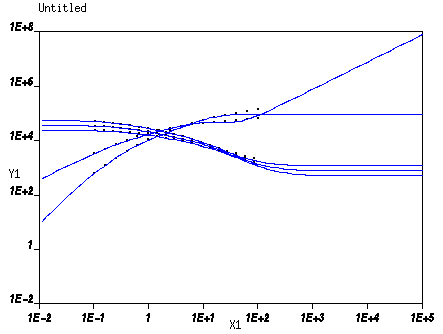
The computed and experimental curves are shown in Figure 10.3: Plot of Computed and Experimental Curves.

Figure 10.3: Plot of Computed and Experimental Curves