10.2.2. Fitting Procedure in Ansys Polymat

Start Ansys Polymat by typing polymat. Then follow the procedure below to perform the fitting for the data presented in Experimental Data.

Note that the fitting calculation for this example will take longer than for the generalized Newtonian example in Example 1: Non-Isothermal Generalized Newtonian Model, due to the added complexity of the model.

10.2.2.1. Step 1: Define the Fluid Model Type

Select Fluid Model

Choose a Differential non-isothermal viscoelastic model.
Differential non-isothermal viscoelastic model
Return to the top-level menu.

10.2.2.2. Step 2: Specify the Material Data Models and Fix Parameters

Material Data

Specify the temperature dependence.
Temperature dependence of viscosity
1. Select the Arrhenius law.
  Arrhenius law
2. Enable the fixing of parameters.
  1. Click the Fix button at the top of the Ansys Polymat menu.
  2. Click OK to confirm that fixing is enabled.
3. Fix the value of to be .
  1. Specify .
    Modify t0
  2. Specify that is fixed.
    t0 is a fixed value
  3. Return to the Arrhenius law menu.
4. Disable the fixing of parameters.
  1. Click the Fix button at the top of the Ansys Polymat menu.
  2. Click OK to confirm that fixing is disabled.
5. Return to the Material Data menu.
Specify the differential viscoelastic models.
Differential viscoelastic models
1. Specify the differential viscoelastic model for the first relaxation mode and fix parameters.
  1-st viscoelastic model
  1. Select the Giesekus model.
    Giesekus model
  2. Accept the current values.
  3. Return to the Differential viscoelastic models menu.
2. Specify the differential viscoelastic model for the second relaxation mode.
  Addition of a viscoelastic model
  1. Select the Giesekus model.
    Giesekus model
  2. Accept the current values.
  3. Return to the Differential viscoelastic models menu.
3. Specify the differential viscoelastic model for the third relaxation mode and fix parameters.
  Addition of a viscoelastic model
  1. Select the Giesekus model.
    Giesekus model
  2. Accept the current values.
  3. Return to the Differential viscoelastic models menu.
Return to the top-level Ansys Polymat menu.

10.2.2.3. Step 3: Read in and Draw the Experimental Data Curves

Enter the Automatic Fitting menu.
Automatic fitting
Enter the List of Experimental Curves menu.
Add experimental curves
Add the first experimental curve (visco_200.crv).
Add a new curve
1. Select the curve named visco_200.crv.
  Enter the name of the curve file
2. Set the reference temperature to 200.
  Modify the temperature
3. Specify that the curve is a shear viscosity curve.
  Modify the curve type
  1. Choose steady shear viscosity (the default).
    steady shear viscosity
  2. Return to the List of Experimental Curves menu.
Add the second experimental curve (visco_220.crv).
Add a new curve
1. Select the curve named visco_220.crv.
  Enter the name of the curve file
2. Set the reference temperature to 220.
  Modify the temperature
3. Specify that the curve is a shear viscosity curve.
  Modify the curve type
  1. Choose steady shear viscosity (the default).
    steady shear viscosity
  2. Return to the List of Experimental Curves menu.
Repeat to add the third shear viscosity curve (visco_240.crv) and set the appropriate reference temperature and curve type.
Add the storage modulus curve (gprime.crv).
Add a new curve
1. Select the curve named gprime.crv.
  Enter the name of the curve file
2. Set the reference temperature to 220.
  Modify the temperature
3. Specify that the curve is a storage modulus curve.
  Modify the curve type
  1. Choose storage modulus G’.
    storage modulus G’
  2. Return to the List of Experimental Curves menu.
Add the loss modulus curve (gsecond.crv).
Add a new curve
1. Select the curve named gsecond.crv.
  Enter the name of the curve file
2. Set the reference temperature to 220.
  Modify the temperature
3. Specify that the curve is a loss modulus curve.
  Modify the curve type
  1. Choose loss modulus G".
    loss modulus G"
  2. Return to the List of Experimental Curves menu.
Return to the Automatic Fitting menu.
Plot the five experimental data curves.
Draw experimental curves

10.2.2.4. Step 4: Set Numerical Options and Run the Fitting Calculation

Set the numerical parameters for the calculation.
Numerical options for fitting
1. Limit the range of relaxation times to be from a minimum of 0.1 to a maximum of 10.
  Modify the range of relaxation times
2. Return to the Automatic Fitting menu.
Specify a name for the material data file (for example, example2.mat).
Enter the name of the result file
Start the fitting calculation.
Run fitting

10.2.2.5. Results

The results of the fitting calculation are as follows:

RESULTS
 
 
 nb. of modes = 3
 
 mode # 1 - Giesekus model
 T = T1 + T2
 (1+alfa*trelax/visc1*T1)*T1 + trelax*T1up = 2*visc1*D
 T2 = 2*visc2*D
 where - visc is the viscosity
       - visc1 = (1-ratio)*visc
       - visc2 = ratio*visc
       - trelax is the relaxation time
       - T1up is the upper-convected time derivative of T1
 
 visc    = 0.8395177E+04 [auto]
 trelax  = 0.1000000E+00 [auto]
 alfa    = 0.5175758E+00 [auto]
 ratio   = 0.8191842E-01 [auto]
 
 mode # 2 - Giesekus model

 T = T1 + T2
 (1+alfa*trelax/visc1*T1)*T1 + trelax*T1up = 2*visc1*D
 T2 = 2*visc2*D
 where - visc is the viscosity
       - visc1 = (1-ratio)*visc
       - visc2 = ratio*visc
       - trelax is the relaxation time
       - T1up is the upper-convected time derivative of T1

 visc   = 0.1901750E+05 [auto]
 trelax = 0.1000000E+01 [auto]
 alfa   = 0.6759477E+00 [auto]
 ratio  = 0.0000000E+00 [fixed]
 
 mode # 3 - Giesekus model

 T = T1 + T2
 (1+alfa*trelax/visc1*T1)*T1 + trelax*T1up = 2*visc1*D
 T2 = 2*visc2*D

 where - visc is the viscosity
       - visc1 = (1-ratio)*visc
       - visc2 = ratio*visc
       - trelax is the relaxation time
       - T1up is the upper-convected time derivative of T1
 
 visc   = 0.9246148E+04 [auto]
 trelax = 0.1000000E+02 [auto]
 alfa   = 0.3902228E+00 [auto]
 ratio  = 0.0000000E+00 [fixed]
 
 Arrhenius law
 h(t) = exp( alfa / (t-t0) - alfa / (talfa-t0) )
 
 alfa   = 0.5019328E+04 [auto]
 talfa  = 0.2200000E+03 [auto]
 t0     = -0.2731500E+03 [fixed]

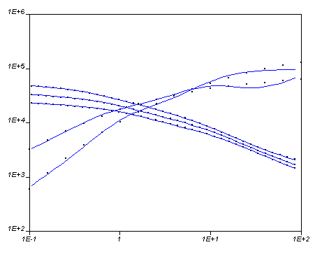
The computed and experimental curves are shown in Figure 10.2: Plot of Computed and Experimental Curves.

Figure 10.2: Plot of Computed and Experimental Curves