


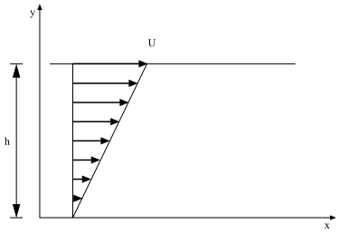
Steady simple shear flow is characterized by a horizontal velocity field, illustrated in Figure 7.1: Steady Simple Shear Flow and defined as follows:
 | (7–1) |
where  ,
,  , and
, and  are the velocity components in the
  ,
,  , and
, and  directions, respectively, and
  is the constant shear rate, which is equal to
  .
.
On the basis of this flow field, the following properties can be computed:
steady shear stress:

(7–2)
In the Load Curves (Part I) menu, click Shear Stress.
steady shear viscosity:

(7–3)
In the Load Curves (Part I) menu, click Shear Viscosity.
first normal-stress difference:

(7–4)
In the Load Curves (Part I) menu, click 1st Normal Stress Difference.
second normal-stress difference:

(7–5)
In the Load Curves (Part I) menu, click 2nd Normal Stress Difference.
first normal-stress coefficient:

(7–6)
In the Load Curves (Part I) menu, click 1st Normal Stress Coefficient.
second normal-stress coefficient:

(7–7)
In the Load Curves (Part I) menu, click 2nd Normal Stress Coefficient.
recoverable stress:

(7–8)
In the Load Curves (Part I) menu, click Stress ratio Sr.
estimated relaxation time:

(7–9)
In the Load Curves (Part I) menu, click Lambda = Sr / shear_rate.
Note: Equation 7–4 — Equation 7–9 have nonzero values only for viscoelastic fluids. For this reason, these properties are not available in Ansys Polymat for generalized Newtonian fluids.
To compute each of these curves, you will need to specify a minimum and maximum shear
rate ( and
and  ), and the number of sampling points. See Defining Numerical Parameters and Defining Numerical Parameters for information about
specifying numerical parameters for viscometric property curves. See Specifying the Curves to be Calculated for information about
specifying which curves you want to compute and plot. (Note that, if you use the
automatic fitting method, Ansys Polymat will automatically compute and plot the curves
for all properties for which experimental data curves have been defined.)
), and the number of sampling points. See Defining Numerical Parameters and Defining Numerical Parameters for information about
specifying numerical parameters for viscometric property curves. See Specifying the Curves to be Calculated for information about
specifying which curves you want to compute and plot. (Note that, if you use the
automatic fitting method, Ansys Polymat will automatically compute and plot the curves
for all properties for which experimental data curves have been defined.)