


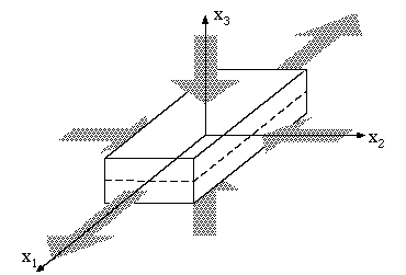
Steady extensional flow can be uniaxial, biaxial, or planar. Uniaxial extensional flow is illustrated in Figure 7.2: Uniaxial Extensional Flow and defined as follows:
 | (7–10) |
where  is a constant elongational strain rate.
The corresponding stress distribution can be written as
 | (7–11) |
 | (7–12) |
where  is the uniaxial extensional viscosity.
Biaxial extensional flow is illustrated in Figure 7.3: Biaxial Extensional Flow and defined as follows:
 | (7–13) |
where  is a constant elongational strain rate.
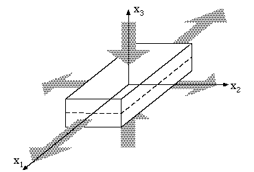
The corresponding stress distribution can be written as
 | (7–14) |
 | (7–15) |
where  is the biaxial extensional viscosity.
Planar extensional flow is illustrated in Figure 7.4: Planar Extensional Flow and defined as follows:
 | (7–16) |
where  is a constant elongational strain rate.
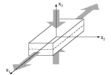
The corresponding stress distribution can be written as
 | (7–17) |
where  is the planar extensional viscosity.
For extensional flow fields, the uniaxial, biaxial, and planar extensional viscosity
curves ( ,
,  , and
, and  ) can be computed. Click Uniaxial Extensional
Viscosity, Biaxial Extensional Viscosity, and/or
Planar Extensional Viscosity in the Load Curves (Part
I) menu if you want Ansys Polymat to compute one (or more) of these
curves.
) can be computed. Click Uniaxial Extensional
Viscosity, Biaxial Extensional Viscosity, and/or
Planar Extensional Viscosity in the Load Curves (Part
I) menu if you want Ansys Polymat to compute one (or more) of these
curves.
To compute each of these curves, you will need to specify a minimum and maximum
extensional strain rate ( and
and  ), and the number of sampling points. See Defining Numerical Parameters and Defining Numerical Parameters for information about
specifying numerical parameters for viscometric property curves. See Specifying the Curves to be Calculated for information about
specifying which curves you want to compute and plot. (Note that, if you use the
automatic fitting method, Ansys Polymat will automatically compute and plot the curves
for all properties for which experimental data curves have been defined.)
), and the number of sampling points. See Defining Numerical Parameters and Defining Numerical Parameters for information about
specifying numerical parameters for viscometric property curves. See Specifying the Curves to be Calculated for information about
specifying which curves you want to compute and plot. (Note that, if you use the
automatic fitting method, Ansys Polymat will automatically compute and plot the curves
for all properties for which experimental data curves have been defined.)