


There are currently nine differential viscosity models:
Upper-convected Maxwell and Oldroyd-B models: These are the simplest viscoelastic constitutive equations, although in many situations they are the most numerically cumbersome for Ansys Polyflow. Both models exhibit a constant viscosity and a quadratic first normal-stress difference. They should be selected either when very little information is know about the fluid, or when a qualitative prediction is sufficient. For fluids exhibiting a very high extensional viscosity, the Oldroyd-B model is preferred over the upper-convected Maxwell model.
White-Metzner model: Most fluids are characterized by shear thinning and a non-quadratic first normal-stress difference. With the White-Metzner model, it is possible to reproduce such viscometric features. Several functions for the shear-rate dependence of the viscosity and the relaxation time are available.
When experimental data are available for the shear viscosity and the first normal-stress difference, the material parameters for the White-Metzner model can be obtained easily by curve fitting: first the shear viscosity is defined and fitted, and then the function for the relaxation time can be selected and fitted on the basis of the first normal-stress difference in a simple shear flow.
Despite its interesting features from a viscometric point of view, the White-Metzner model may exhibit strange numerical behavior at high shear rates, leading to spurious oscillations in the Ansys Polyflow solution.
Phan-Thien-Tanner (PTT), Johnson-Segalman, and Giesekus models: These models are the most realistic. In particular, they exhibit shear thinning and a non-quadratic first normal-stress difference at high shear rates. These properties are controlled by their respective material parameters (
 ,
,  , and
, and  ), as described in the model description below. Also, the
selection of nonzero values for
), as described in the model description below. Also, the
selection of nonzero values for  and
and  will lead to a bounded steady extensional viscosity.
 For stability reasons, however, a purely viscous component must be added to the extra-stress tensor in simple shear flow. This is true for the Johnson-Segalman and PTT models when
 is nonzero, and for the Giesekus model when
 >0.5. The addition of a purely viscous component to the
extra-stress tensor affects the viscosity, but not the first normal-stress
difference. Shear thinning is still present, but the viscosity curve also
shows a plateau zone at high shear rates.
>0.5. The addition of a purely viscous component to the
extra-stress tensor affects the viscosity, but not the first normal-stress
difference. Shear thinning is still present, but the viscosity curve also
shows a plateau zone at high shear rates. Poor control of the shear viscosity is the usual drawback of the Johnson-Segalman and PTT models used with a single relaxation time, especially toward high shear rates.
Important: Note that you cannot explicitly select the Johnson-Segalman model in the Ansys Polymat interface. It is obtained by selecting the PTT model and setting the value of
 to 0.
to 0.FENE-P (Finitely Extensible Non-Linear Elastic Dumbbells – Peterlin) model: This model is derived from molecular theories and is based on the assumption that the material behaves as a series of dumbbells linked together by springs. Unlike the Maxwell model, springs can have only a finite extension, so the energy of deformation of the dumbbell becomes infinite for a finite value of the spring elongation.
The FENE-P model requires only four parameters (
 ,
,  ,
,  , and the length ratio for the spring), yet it predicts a
realistic shear thinning of the fluid and a first normal-stress difference
that is quadratic for low shear rates and has a lower slope for high shear
rates. It has been observed in practice that viscometric properties of
several fluids can often be accurately modeled. The FENE-P model is well
suited for simulating the rheological behavior of dilute solutions.
, and the length ratio for the spring), yet it predicts a
realistic shear thinning of the fluid and a first normal-stress difference
that is quadratic for low shear rates and has a lower slope for high shear
rates. It has been observed in practice that viscometric properties of
several fluids can often be accurately modeled. The FENE-P model is well
suited for simulating the rheological behavior of dilute solutions. POM-POM model: The pom-pom molecule consists of a backbone to which
 arms are connected at both extremities. In a flow, the
backbone may orient in a Doi-Edwards reptation tube consisting of the
neighboring molecules, while the arms may retract into that tube. The
concept of the pom-pom macromolecule makes the model suitable for describing
the behavior of branched polymers. The approximate differential form of the
model is based on the equations of macromolecular orientation and
macromolecular stretching in connection with changes in orientation. In this
construction, the pom-pom molecule is allowed only a finite extension, which
is controlled by the number of dangling arms. In particular, the strain
hardening properties are dictated by the number of arms. Beyond that, the
model predicts realistic shear thinning behavior, as well as a first and a
possible second normal stress difference.
arms are connected at both extremities. In a flow, the
backbone may orient in a Doi-Edwards reptation tube consisting of the
neighboring molecules, while the arms may retract into that tube. The
concept of the pom-pom macromolecule makes the model suitable for describing
the behavior of branched polymers. The approximate differential form of the
model is based on the equations of macromolecular orientation and
macromolecular stretching in connection with changes in orientation. In this
construction, the pom-pom molecule is allowed only a finite extension, which
is controlled by the number of dangling arms. In particular, the strain
hardening properties are dictated by the number of arms. Beyond that, the
model predicts realistic shear thinning behavior, as well as a first and a
possible second normal stress difference. Leonov model: This model has been developed for the simultaneous prediction of the behavior of trapped and free macromolecular chains for filled elastomers with carbon black and/or silicate. From the point of view of morphology, macromolecules at rest are trapped by particles of carbon black, via electrostatic van der Waals forces. Under a deformation field, electrostatic bonds can break, and macromolecules become free, while a reverse mechanism may develop when the deformation ceases. You can therefore be facing a macromolecular system consisting of trapped and free macromolecules, with a reversible transition from one state to the other one.
This model involves actually two tensor quantities and a scalar one. The tensors focus respectively on the behavior of the free and trapped macromolecular chains of the elastomer, while the scalar quantity quantifies the degree of structural damage (debonding factor). The model exhibits a yielding behavior. It is intrinsically nonlinear, as the nonlinear response develops and is observable at early deformations.
Details about each model are provided below.
The Maxwell model is one of the simplest viscoelastic constitutive equations. It exhibits a constant viscosity and a quadratic first normal-stress difference. Due to its simplicity, it is recommended only when little information about the fluid is available, or when a qualitative prediction is sufficient. Even in this case, the Oldroyd-B model, which can include a purely viscous component, is preferable for numerical reasons.
For the upper-convected Maxwell model, the purely viscous component of the
extra-stress tensor ( ) is equal to zero. The viscoelastic component
(
) is equal to zero. The viscoelastic component
( ) is computed from
 | (6–30) |
where  is a model-specific relaxation time,
  is the rate-of-deformation tensor, and
  is a model-specific viscosity factor for the viscoelastic
component of
is a model-specific viscosity factor for the viscoelastic
component of  . The relaxation time
  is defined as the time required for the shear stress to be
reduced to half of its original equilibrium value when the strain rate
vanishes. A high relaxation time indicates that the memory retention of the
flow is high. A low relaxation time indicates significant memory loss,
gradually approaching Newtonian flow (zero relaxation time).
is defined as the time required for the shear stress to be
reduced to half of its original equilibrium value when the strain rate
vanishes. A high relaxation time indicates that the memory retention of the
flow is high. A low relaxation time indicates significant memory loss,
gradually approaching Newtonian flow (zero relaxation time).
The units for the parameters and their names in the Ansys Polymat interface are as follows:
| Parameter | Name in Ansys Polymat | Mass | Length | Time |
|---|---|---|---|---|

| visc | 1 | –1 | –1 |

| trelax | – | – | 1 |

| – | 1 | –1 | –2 |

| – | – | – | –1 |
By default,  and
and  are equal to 1.
Figure 6.28: Upper-Convected Maxwell Model for a Shear Flow
shows the viscometric functions of the upper-convected Maxwell model in a
simple shear flow. In this example (where  =1 s and
  =1000 Pa-s),
  is constant,
  is linear,
  is quadratic,
  is zero,
  is constant,
  is zero, and
  is linear, showing non-asymptotic behavior.
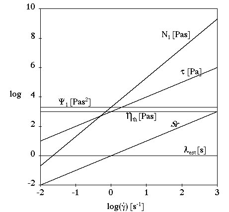
Figure 6.29: Upper-Convected Maxwell Model for an Extensional Flow shows the behavior of the upper-convected Maxwell model in a simple extensional flow.
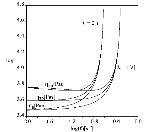
In this example (where  =1 s and
  =1000 Pa-s),
  ,
,  , and
, and  are unbounded for
  , and
, and
 | (6–31) |
 | (6–32) |
 | (6–33) |
 | (6–34) |
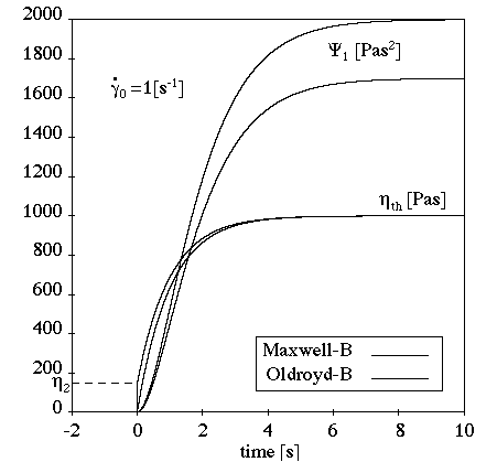
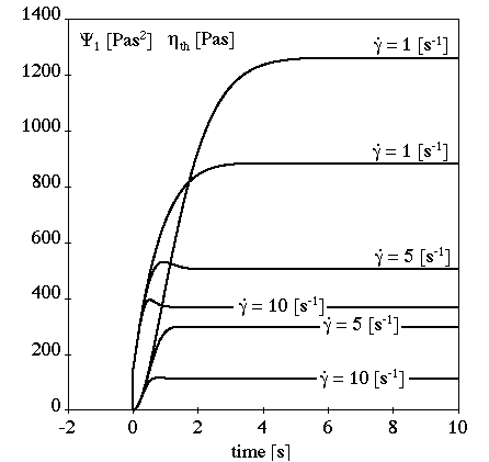
Figure 6.30: Upper-Convected Maxwell Model for a Transient Shear Flow shows the behavior of the upper-convected Maxwell model in a transient shear flow.
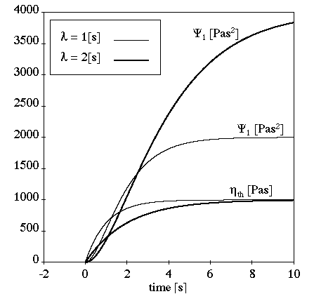
In this example (where  =1 s,
=1 s,  =1000 Pa-s, and
  s-1), there is no stress
overshoot and the transient phase depends upon the relaxation time.
s-1), there is no stress
overshoot and the transient phase depends upon the relaxation time.
The Oldroyd-B model is, like the Maxwell model, one of the simplest viscoelastic constitutive equations. It is slightly better than the Maxwell model, because it allows for the inclusion of the purely viscous component of the extra stress, which leads to better behavior of the numerical scheme. Oldroyd-B is a good choice for fluids that exhibit a very high extensional viscosity.
For the Oldroyd-B model,  is computed from Equation 6–30,
and
is computed from Equation 6–30,
and  is computed (optionally) from Equation 6–27.
 in Equation 6–30, and
  in Equation 6–27 are partial shear viscosities. Ansys Polymat uses
Equation 6–28
and Equation 6–29
to compute the value of
in Equation 6–27 are partial shear viscosities. Ansys Polymat uses
Equation 6–28
and Equation 6–29
to compute the value of  , based on a specified value for the viscosity ratio,
 .
.
The units for the parameters and their names in the Ansys Polymat interface are as follows:
| Parameter | Name in Ansys Polymat | Mass | Length | Time |
|---|---|---|---|---|

| visc | 1 | –1 | –1 |

| trelax | – | – | 1 |

| ratio | – | – | – |

| – | 1 | –1 | –2 |

| – | – | – | –1 |
By default,  and
and  are equal to 1, and the viscosity ratio
  is equal to 0 (that is,
  and
and  are equal to 0).
Figure 6.31: Oldroyd-B Model for a Shear Flow shows
the viscometric functions of the Oldroyd-B model in a simple shear flow. In
this example,  =1 s and (with the viscosity ratio equal to 0.15)
 =850 Pa-s and
  =150 Pa-s. In the resulting curves,
  is constant,
  is linear,
  is quadratic,
  is zero,
  is constant,
  is zero, and
  is linear, showing non-asymptotic behavior. Notice that
the curves are moved down in comparison to the upper-convected Maxwell
model; this is due to the Newtonian part of the model (nonzero value for
is linear, showing non-asymptotic behavior. Notice that
the curves are moved down in comparison to the upper-convected Maxwell
model; this is due to the Newtonian part of the model (nonzero value for
 ), which reduces the viscoelastic effects (
 ,
,  ,
,  , and
, and  ).
).
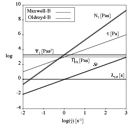
Figure 6.32: Oldroyd-B Model for a Transient Shear Flow shows
the behavior of the Oldroyd-B model in a transient shear flow. In this
example,  =1 s,
=1 s,  =1000 Pa-s, and
  s–1. Notice that
there is an instantaneous response of the shear stress to the applied shear
rate; this is due to the Newtonian part of the model. Otherwise, the
Oldroyd-B model exhibits the same behavior as the upper-convected Maxwell
model.
s–1. Notice that
there is an instantaneous response of the shear stress to the applied shear
rate; this is due to the Newtonian part of the model. Otherwise, the
Oldroyd-B model exhibits the same behavior as the upper-convected Maxwell
model.
Most fluids are characterized by shear-thinning and non-quadratic first normal-stress difference. With the White-Metzner model, it is possible to reproduce such viscometric features.
The White-Metzner model computes  from
from
 | (6–35) |
and  is computed (optionally) from Equation 6–27.
 in Equation 6–35 and
  in Equation 6–27 are partial shear viscosities.
The relaxation time ( ) and the viscosity (
 ) can be constant or represented by the power law or the
Bird-Carreau law for shear-rate dependence.
) can be constant or represented by the power law or the
Bird-Carreau law for shear-rate dependence.
The power-law representation of the total viscosity is
 | (6–36) |
where  is the consistency factor,
  is the power-law index, and
  is the natural time (that is, inverse of the shear rate at
which the fluid changes from Newtonian to power-law behavior).
is the natural time (that is, inverse of the shear rate at
which the fluid changes from Newtonian to power-law behavior).
The Bird-Carreau representation of the viscosity is
 | (6–37) |
where  is the natural time and
  is the power-law index.
 and
and  are then computed from Equation 6–28 and
Equation 6–29,
based on a specified value for the viscosity ratio,
are then computed from Equation 6–28 and
Equation 6–29,
based on a specified value for the viscosity ratio,  .
.
The power-law representation of the relaxation time is
 | (6–38) |
The Bird-Carreau representation of the relaxation time is
 | (6–39) |
Important: Note that the power-law representation for the relaxation time should be avoided, since it leads to high relaxation times for low shear rates. The Bird-Carreau representation is better, yielding a constant (and bounded) relaxation time at low shear rates.
If you are fitting experimental curves using the White-Metzner model, you will need to do the fitting in two parts:
Choose the viscosity function and fit its parameters. See Shear-Rate Dependence of Viscosity for information about the parameters for the function you choose (constant, Bird-Carreau, or power law).
Choose the relaxation time function and fit its parameters to the experimental curve for the first normal-stress difference. See Shear-Rate Dependence of Viscosity for information about the parameters for the function you choose (constant, Bird-Carreau, or power law). Note that the relaxation time function has no effect on the steady viscosity curves.
The units for the White-Metzner parameters and their names in the Ansys Polymat interface are as follows:
| Parameter | Name in Ansys Polymat | Mass | Length | Time |
|---|---|---|---|---|

| viscosity function | 1 | –1 | –1 |

| relaxation time function | – | – | 1 |

| ratio | – | – | – |

| – | 1 | –1 | –2 |

| – | – | – | –1 |
By default,  and
and  are constant values equal to 1, and the viscosity ratio
 is equal to 0 (that is,
  and
and  are equal to 0).
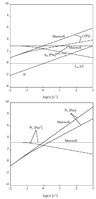
Figure 6.33: White-Metzner Model for a Shear Flow compares the White-Metzner model to the
upper-convected Maxwell model for a simple shear flow. In this example, the
Bird-Carreau viscosity law is used, with  =1000 Pa-s,
  =10 s, and
  =0.5. The relaxation time
  is 1 s. Notice that
  and
and  are non-constant for large shear rates,
  is nonlinear,
  is non-quadratic for large shear rates, and
 and
and  are equal to 0.
In transient shear flow, the White-Metzner model is similar in behavior to the upper-convected Maxwell model. The shape of the curves is the same, but the duration of the transient phase depends on the relaxation time function. If this function is constant, the duration to reach the regime situation is the same; if it is not constant, the duration of the transient phase depends upon the relaxation time function. Usually, the relaxation time is a decreasing function of the shear rate, so the duration of the transient phase is reduced for high shear rate.
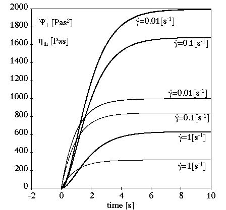
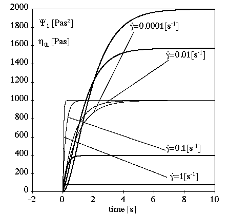
Figure 6.34: White-Metzner Model for a Transient Shear Flow with Constant Relaxation Time shows the viscometric curves for a constant relaxation time and Figure 6.35: White-Metzner Model for a Transient Shear Flow with a Bird-Carreau Relaxation Time shows the curves for a shear-rate-dependent relaxation time. In Figure 6.34: White-Metzner Model for a Transient Shear Flow with Constant Relaxation Time, the shear thinning affects the final value of the viscosity and the first normal-stress coefficient. The transient phase is not affected by the shear rate. In Figure 6.35: White-Metzner Model for a Transient Shear Flow with a Bird-Carreau Relaxation Time, there is no shear thinning, so there is no effect on the final value of the viscosity. The first normal stress coefficient is affected by the variation of relaxation time with shear rate. The transient phase is affected by the shear rate.
The Phan-Thien-Tanner (PTT) model is one of the most realistic differential viscoelastic models. It exhibits shear thinning and a non-quadratic first normal-stress difference at high shear rates.
The PTT model computes  from
from
 | (6–40) |
and  is computed (optionally) from Equation 6–27.
 in Equation 6–40 and
  in Equation 6–27 are partial shear viscosities. Ansys Polymat uses
Equation 6–28
and Equation 6–29
to compute the value of
in Equation 6–27 are partial shear viscosities. Ansys Polymat uses
Equation 6–28
and Equation 6–29
to compute the value of  , based on a specified value for the viscosity ratio,
 .
.
 and
and  are material properties that control, respectively, the
shear viscosity and elongational behavior. A nonzero value for
are material properties that control, respectively, the
shear viscosity and elongational behavior. A nonzero value for
 leads to a bounded steady extensional viscosity.
The units for the parameters and their names in the Ansys Polymat interface are as follows:
| Parameter | Name in Ansys Polymat | Mass | Length | Time |
|---|---|---|---|---|

| visc | 1 | –1 | –1 |

| trelax | – | – | 1 |

| ratio | – | – | – |

| eps | – | – | – |

| xi | – | – | – |

| – | 1 | –1 | –2 |

| – | – | – | –1 |
By default,  and
and  are equal to 1, the viscosity ratio
  is equal to 0 (that is,
  and
and  are equal to 0), and
  and
and  are also equal to 0. Note that when
  =0, the PTT model is reduced to the Johnson-Segalman model.
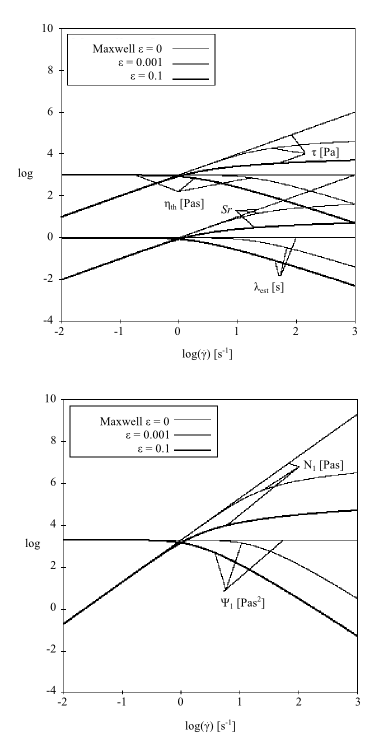
In a simple shear flow (Figure 6.36: PTT Model for a Shear Flow), for  >0, you can see a shear-thinning effect and a
non-quadratic behavior for the first normal-stress difference
>0, you can see a shear-thinning effect and a
non-quadratic behavior for the first normal-stress difference
 . Notice also that, for
  >0, the elasticity level
  remains finite for increasing shear rate (asymptotic
behavior).
remains finite for increasing shear rate (asymptotic
behavior).
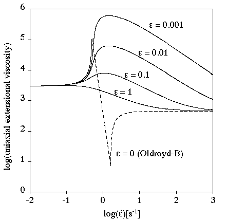
The parameter  also affects the extensional viscosities, as shown in
Figure 6.37: PTT Model for a Steady Extensional Flow.
The steady extensional viscosities are finite, and tend toward the Newtonian
component of the extensional viscosity (that is, they are uniaxial) for
large extension rates. For small values of
also affects the extensional viscosities, as shown in
Figure 6.37: PTT Model for a Steady Extensional Flow.
The steady extensional viscosities are finite, and tend toward the Newtonian
component of the extensional viscosity (that is, they are uniaxial) for
large extension rates. For small values of  , there is extension thickening and thinning; for large
values, there is only extension thinning.
, there is extension thickening and thinning; for large
values, there is only extension thinning.
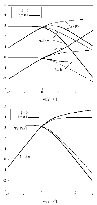
Important: If the parameter  is not zero, then the viscosity ratio
  must be at least 1/9, in order to ensure the stability
of the shear flow. However, this value may decrease when does not vanish. The slope of the shear stress
vs. shear rate curve must be positive everywhere, contrary to what
is shown on the left in Figure 6.38: Effect of ξ on the PTT Model for a Shear Flow with
must be at least 1/9, in order to ensure the stability
of the shear flow. However, this value may decrease when does not vanish. The slope of the shear stress
vs. shear rate curve must be positive everywhere, contrary to what
is shown on the left in Figure 6.38: Effect of ξ on the PTT Model for a Shear Flow with  =0.1.
=0.1.
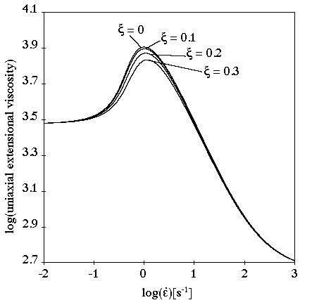
The parameter  has almost no effect on extensional viscosity, as shown in
Figure 6.39: Effect of ξ on the PTT Model for a Steady Extensional
Flow. The maximum of the extensional viscosities decreases when
has almost no effect on extensional viscosity, as shown in
Figure 6.39: Effect of ξ on the PTT Model for a Steady Extensional
Flow. The maximum of the extensional viscosities decreases when
 increases.
In a transient shear flow (Figure 6.40: PTT Model in a Transient Shear Flow), a moderate stress overshoot is observed. The stress overshoot increases as shear rate increases. Shear thinning is observed, and the normal stress is non-quadratic. The transient phase is reduced as the shear rate increases.
Like the PTT model, the Giesekus model is one of the most realistic differential viscoelastic models. It exhibits shear thinning and a non-quadratic first normal-stress difference at high shear rates.
The Giesekus model computes  from
from
 | (6–41) |
and  is computed (optionally) from Equation 6–27.
 in Equation 6–41 and
  in Equation 6–27 are partial shear viscosities. Ansys Polymat uses
Equation 6–28
and Equation 6–29
to compute the value of
in Equation 6–27 are partial shear viscosities. Ansys Polymat uses
Equation 6–28
and Equation 6–29
to compute the value of  , based on a specified value for the viscosity ratio,
 .
.
 is the unit tensor and
  is a material constant that controls the extensional
viscosity and the ratio of the second normal-stress difference to the first.
For low values of shear rate,
is a material constant that controls the extensional
viscosity and the ratio of the second normal-stress difference to the first.
For low values of shear rate,
 | (6–42) |
For the majority of fluids, this ratio is between 0.1 and 0.2.
The units for the parameters and their names in the Ansys Polymat interface are as follows:
| Parameter | Name in Ansys Polymat | Mass | Length | Time |
|---|---|---|---|---|

| visc | 1 | –1 | –1 |

| trelax | – | – | 1 |

| ratio | – | – | – |

| alfa | – | – | – |

| – | 1 | –1 | –2 |

| – | – | – | –1 |
By default,  and
and  are equal to 1, the viscosity ratio
  is equal to 0 (that is,
  and
and  are equal to 0), and
  is also equal to 0.
In a simple shear flow (Figure 6.41: Giesekus Model for a Shear Flow),
 controls the shear-thinning effect. The first
normal-stress difference is non-quadratic, and the cut-off appears earlier
if
controls the shear-thinning effect. The first
normal-stress difference is non-quadratic, and the cut-off appears earlier
if  increases. If
  >0.5, you must add a Newtonian component
(
>0.5, you must add a Newtonian component
( ) to the total viscosity in order to avoid instabilities.
Figure 6.42: Effect of α on the Giesekus Model for an Extensional Flow shows the behavior of the Giesekus fluid in an extensional flow.
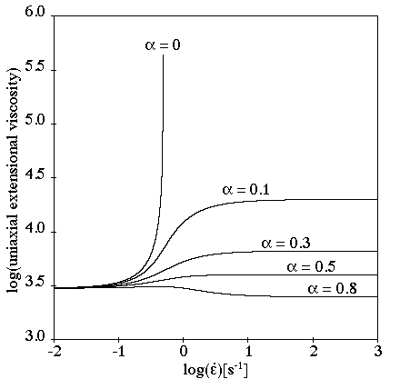
Here, the steady extensional viscosities are finite. For small values of
 extension thickening occurs, and for large values
extension thinning occurs.
extension thickening occurs, and for large values
extension thinning occurs.
In a transient shear flow (Figure 6.43: Giesekus Model for a Transient Shear Flow), the stress overshoot is less severe than for the PTT model; there are fewer oscillations.
The duration of the transient phase depends on the imposed shear rate (the same behavior as for the PTT model). For a high shear rate, the stress overshoots during the transient phase. As the shear rate increases, the final value decreases as the overshoot increases. The duration of the transient phases decreases as the shear rate increases.
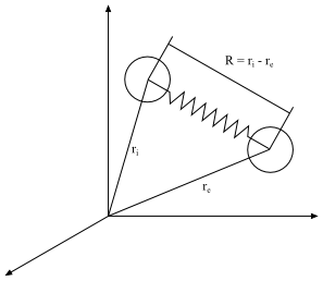
The FENE-P model is derived from molecular theories and is based on the
assumption that the polymer macromolecules are idealized as dumbbells linked
with an elastic connector or spring and suspended in a Newtonian solvent of
viscosity  . Unlike in the Maxwell model, however, the springs are allowed
only a finite extension, so that the energy of deformation of the dumbbell
becomes infinite for a finite value of the spring elongation. This model
predicts a realistic shear thinning of the fluid and a first normal-stress
difference that is quadratic for low shear rates and has a lower slope for high
shear rates.
. Unlike in the Maxwell model, however, the springs are allowed
only a finite extension, so that the energy of deformation of the dumbbell
becomes infinite for a finite value of the spring elongation. This model
predicts a realistic shear thinning of the fluid and a first normal-stress
difference that is quadratic for low shear rates and has a lower slope for high
shear rates.
The FENE-P model computes  from
from
 | (6–43) |
where  is computed from
 | (6–44) |
and  is the ratio of the maximum length of the spring to its
length at rest:
is the ratio of the maximum length of the spring to its
length at rest:
 | (6–45) |
 is an equilibrium length that corresponds to rigid motion
(in this case,
is an equilibrium length that corresponds to rigid motion
(in this case,  =0 and the tension in the connector equals the Brownian
forces).
=0 and the tension in the connector equals the Brownian
forces).  is the maximum allowable dumbbell length. Figure 6.44: Dumbbell Definitions for the FENE-P Model shows how
the distance between dumbbells is based on the relative position of both
ends.
is the maximum allowable dumbbell length. Figure 6.44: Dumbbell Definitions for the FENE-P Model shows how
the distance between dumbbells is based on the relative position of both
ends.
 is always greater than 1. As
  becomes infinite, the FENE-P model reduces to the
upper-convected Maxwell model.
becomes infinite, the FENE-P model reduces to the
upper-convected Maxwell model.
 is computed (optionally) from Equation 6–27.
 in Equation 6–43 and
  in Equation 6–27 are partial shear viscosities. Ansys Polymat uses
Equation 6–28 and Equation 6–29 to compute the value of
in Equation 6–27 are partial shear viscosities. Ansys Polymat uses
Equation 6–28 and Equation 6–29 to compute the value of
 , based on a specified value for the viscosity ratio,
 .
.
The motion of the dumbbells is the result of hydrodynamic, Brownian, and
spring forces.  represents the tension in the spring (spring forces) and
the Brownian motion.
represents the tension in the spring (spring forces) and
the Brownian motion.  represents the Newtonian (hydrodynamic) forces.
See [1] for additional information about the FENE-P model. Note that the FENE-P model is not available for non-isothermal flows.
The units for the parameters and their names in the Ansys Polymat interface are as follows:
| Parameter | Name in Ansys Polymat | Mass | Length | Time |
|---|---|---|---|---|

| visc | 1 | –1 | –1 |

| trelax | – | – | 1 |

| ratio | – | – | – |

| Lsqrd | – | 2 | – |

| – | 1 | –1 | –2 |

| – | – | – | –1 |
By default,  ,
,  , and
, and  are equal to 1, and the viscosity ratio
  is equal to 0 (that is,
  and
and  are equal to 0).
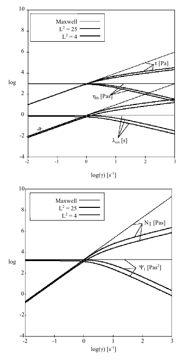
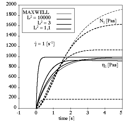
The behavior of the FENE-P model with small values of  for a simple shear flow is illustrated in Figure 6.45: Effect of Small Values of L^2 on the FENE-P Model for Shear
Flow.
Shear thinning occurs with this model, and for large values of shear rate,
the slope is –2/3. Therefore the addition of a Newtonian viscosity
component is not required for stability. The first normal-stress difference
is non-quadratic, and the second normal-stress difference is 0. The cut-off
appears sooner when
for a simple shear flow is illustrated in Figure 6.45: Effect of Small Values of L^2 on the FENE-P Model for Shear
Flow.
Shear thinning occurs with this model, and for large values of shear rate,
the slope is –2/3. Therefore the addition of a Newtonian viscosity
component is not required for stability. The first normal-stress difference
is non-quadratic, and the second normal-stress difference is 0. The cut-off
appears sooner when  decreases, down to a value of 3. No asymptotic behavior is
observed. For low values of shear rate,
decreases, down to a value of 3. No asymptotic behavior is
observed. For low values of shear rate,  decreases as
  decreases.
The behavior of the FENE-P model with large values of  for a simple shear flow is illustrated in Figure 6.46: Effect of Large Values of L^2 on the FENE-P Model for Shear
Flow.
for a simple shear flow is illustrated in Figure 6.46: Effect of Large Values of L^2 on the FENE-P Model for Shear
Flow.
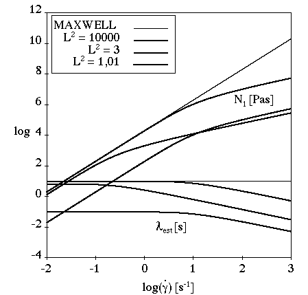
For large values of  , the FENE-P model is observed to exhibit Maxwellian
behavior: quadratic first normal-stress difference and
, the FENE-P model is observed to exhibit Maxwellian
behavior: quadratic first normal-stress difference and  close to
  . For
. For  close to 1, Newtonian behavior is observed: quadratic but
small first normal-stress difference,
close to 1, Newtonian behavior is observed: quadratic but
small first normal-stress difference,  tends toward 0, cut-off occurs at high shear rates. For
low shear rates,
tends toward 0, cut-off occurs at high shear rates. For
low shear rates,
 | (6–46) |
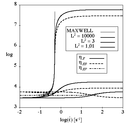
For extensional flows,  controls the extensional viscosity. As shown in Figure 6.47: Effect of L^2 on the FENE-P Model for Extensional Flow, the
extensional viscosities are finite. For large values of
controls the extensional viscosity. As shown in Figure 6.47: Effect of L^2 on the FENE-P Model for Extensional Flow, the
extensional viscosities are finite. For large values of  , the FENE-P model is observed to exhibit Maxwellian
behavior: the extensional viscosities are very high for
, the FENE-P model is observed to exhibit Maxwellian
behavior: the extensional viscosities are very high for  . For
. For  close to 1, Newtonian behavior is observed: the
extensional viscosities are constant.
close to 1, Newtonian behavior is observed: the
extensional viscosities are constant.
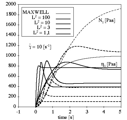
The behavior of the FENE-P model for a transient shear flow is shown in
Figure 6.48: Effect of Large Values of L^2 on the FENE-P Model for Transient Shear
Flow
and Figure 6.49: Effect of Mid-Range Values of L^2 on the FENE-P Model for Transient
Shear Flow.
For high shear rates, the stress overshoots in the transient phase. When the
shear rate increases, the final value and the transient phase decrease while
the overshoot increases. For large values of  , the FENE-P model is observed to exhibit Maxwellian
behavior: no stress overshoots. For mid-range values of
, the FENE-P model is observed to exhibit Maxwellian
behavior: no stress overshoots. For mid-range values of  , the stress overshoots increase and the transient phase
decreases as
, the stress overshoots increase and the transient phase
decreases as  decreases. For
  close to 1, Newtonian behavior is observed: no stress
overshoots and a short transient phase even for high values of shear rate.
close to 1, Newtonian behavior is observed: no stress
overshoots and a short transient phase even for high values of shear rate.
In the POM-POM model, the pom-pom molecule consists of a backbone to which
 arms are connected at both extremities. In a flow, the
backbone may orient in a Doi-Edwards reptation tube consisting of the
neighboring molecules, while the arms may retract into that tube. The concept of
the pom-pom macromolecule makes the model suitable for describing the behavior
of branched polymers. The approximate differential form of the model is based on
equations of macromolecular orientation, and macromolecular stretching in
relation to changes in orientation.
arms are connected at both extremities. In a flow, the
backbone may orient in a Doi-Edwards reptation tube consisting of the
neighboring molecules, while the arms may retract into that tube. The concept of
the pom-pom macromolecule makes the model suitable for describing the behavior
of branched polymers. The approximate differential form of the model is based on
equations of macromolecular orientation, and macromolecular stretching in
relation to changes in orientation.
The model, referred to as DCPP ([2],
[8]), allows for a nonzero second normal
stress difference. The DCPP model computes  from an orientation tensor,
  and a stretching scalar
  (states variables), on the basis of the following algebraic
equation:
(states variables), on the basis of the following algebraic
equation:
 | (6–47) |
where  is the shear modulus and
  is a nonlinear material parameter (the nonlinear material
parameter will be introduced later on). The state variables
is a nonlinear material parameter (the nonlinear material
parameter will be introduced later on). The state variables  and
and  are computed from the following differential equations:
 | (6–48) |
 | (6–49) |
In these equations,  and
and  are the relaxation times associated with the orientation and
stretching mechanisms respectively. In the last equation,
are the relaxation times associated with the orientation and
stretching mechanisms respectively. In the last equation,  characterizes the number of dangling arms (or priority) at the
extremities of the pom-pom molecule or segment. It is an indication of the
maximum stretching that the molecule can undergo, and therefore of a possible
strain hardening behavior.
characterizes the number of dangling arms (or priority) at the
extremities of the pom-pom molecule or segment. It is an indication of the
maximum stretching that the molecule can undergo, and therefore of a possible
strain hardening behavior.  can be obtained from the elongational behavior.
 is a nonlinear parameter that has enabled the introduction of
a non-vanishing second normal stress difference in the DCPP model.
is a nonlinear parameter that has enabled the introduction of
a non-vanishing second normal stress difference in the DCPP model.
A multi-mode DCPP model can also be defined. Each contribution  will involve an orientation tensor
  and a stretching variable
  . A few guidelines are required for the determination of the
several linear and nonlinear parameters.
. A few guidelines are required for the determination of the
several linear and nonlinear parameters.
Consider a multi-mode DCPP model characterized by  modes sorted with increasing values of relaxation times
 (increasing seniority). The linear parameters
  and
and  characterizing the linear viscoelastic behavior of the model
can be determined with the usual procedure.
characterizing the linear viscoelastic behavior of the model
can be determined with the usual procedure.
Then the relaxation times ( ) for stretching should be determined. Depending on the average
number of entanglements of backbone section, the ratio
) for stretching should be determined. Depending on the average
number of entanglements of backbone section, the ratio  should be within the range of 2 to 10. For a completely
unentangled polymer segment, you may accept the physical limit of
should be within the range of 2 to 10. For a completely
unentangled polymer segment, you may accept the physical limit of
 =
= .
.  should also satisfy the constraint
  , since
  sets the fundamental diffusion time for the branch point
controlling the relaxation of polymer segment (
sets the fundamental diffusion time for the branch point
controlling the relaxation of polymer segment ( ).
).
The parameter  indicating the number of dangling arms (or priority) at the
extremities of a pom-pom segment
indicating the number of dangling arms (or priority) at the
extremities of a pom-pom segment  , also indicates the maximum stretching that can be undergone
by that segment, and therefore its possible strain hardening behavior. For a
multi-mode DCPP model, both seniority and priority are assumed to increase
together towards the inner segments; hence
, also indicates the maximum stretching that can be undergone
by that segment, and therefore its possible strain hardening behavior. For a
multi-mode DCPP model, both seniority and priority are assumed to increase
together towards the inner segments; hence  should also increase with
  . The parameter
  can be obtained from the elongational behavior.
 is a fifth set of nonlinear parameters that control the ratio
of second to first normal stress differences. The value of parameter
is a fifth set of nonlinear parameters that control the ratio
of second to first normal stress differences. The value of parameter
 should range between 0 and 1. For moderate values,
 corresponds to twice the ratio of the second to the first
normal stress difference, and may decrease with increasing seniority.
corresponds to twice the ratio of the second to the first
normal stress difference, and may decrease with increasing seniority.
As for other viscoelastic models, a purely viscous component  can be added to the viscoelastic component
  , in order to get the total extra-stress tensor:
 | (6–50) |
where
 | (6–51) |
where  is the rate-of-deformation tensor and
  is the viscosity.
The units for the parameters and their names in the Ansys Polymat interface are as follows:
| Parameter | Name in Ansys Polymat | Mass | Length | Time |
|---|---|---|---|---|

| visc2 | 1 | –1 | –1 |

| trelax | - | - | 1 |

| G0 | 1 | –1 | –2 |

| tlambda | - | - | 1 |

| nbarms | - | - | - |

| xi | - | - | - |
 , ,  , , 
| - | 1 | –1 | –2 |

| - | - | - | –1 |

| - | - | - | - |

| - | - | - | - |
By default,  and
and  are set to 1, the number of arms
  to 2 and the other parameters to 0.
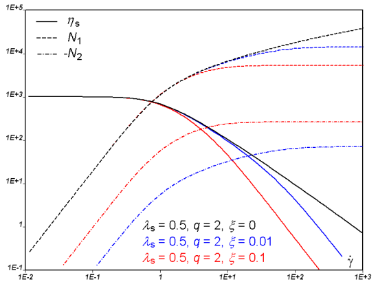
Figure 6.50: Effect of Parameter ξ for Steady Shear Flow shows the
steady viscometric behavior of a single mode DCPP fluid model for various
values of the parameter  . For the present illustration, the shear modulus equals
1000, while the relaxation times for orientation and stretching have been
assigned the values 1 and 0.5, respectively. As can be seen, constant
viscosity and quadratic first normal stress difference are obtained at low
shear rates. Nonlinear behavior is found beyond
. For the present illustration, the shear modulus equals
1000, while the relaxation times for orientation and stretching have been
assigned the values 1 and 0.5, respectively. As can be seen, constant
viscosity and quadratic first normal stress difference are obtained at low
shear rates. Nonlinear behavior is found beyond  . We also find that an increasing value of
  enforces the nonlinear behavior, while it also generates a
non-vanishing second normal stress difference. The other nonlinear
parameters
enforces the nonlinear behavior, while it also generates a
non-vanishing second normal stress difference. The other nonlinear
parameters  and
and  have actually a negligible influence on the viscometric
properties.
have actually a negligible influence on the viscometric
properties.
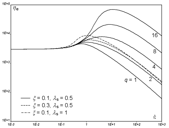
In Figure 6.51: Effect of Parameter q on Steady Elongation Viscosity, we
display the steady elongation viscosity of a single mode DCPP fluid model
for increasing values of  . For the continuous curves, the shear modulus equals 1000,
while the relaxation times for orientation and stretching have been assigned
the values 1 and 0.5, respectively. Also, the nonlinear parameter
. For the continuous curves, the shear modulus equals 1000,
while the relaxation times for orientation and stretching have been assigned
the values 1 and 0.5, respectively. Also, the nonlinear parameter
 is equal to 0.1. As is known for the DCPP model, and more
generally for pom-pom models, the parameter
is equal to 0.1. As is known for the DCPP model, and more
generally for pom-pom models, the parameter  is an indication of branching, and therefore of strain
hardening in elongation. As can be seen from Figure 6.51: Effect of Parameter q on Steady Elongation Viscosity, the
elongation viscosity increases when the strain
is an indication of branching, and therefore of strain
hardening in elongation. As can be seen from Figure 6.51: Effect of Parameter q on Steady Elongation Viscosity, the
elongation viscosity increases when the strain  rate is larger than
  , and the strain hardening is enhanced for increasing
values of
, and the strain hardening is enhanced for increasing
values of  . The figure also shows the steady elongation viscosity
obtained for
. The figure also shows the steady elongation viscosity
obtained for  as well as for
  . As can be seen, the influence of these parameters on the
steady elongation viscosity remains moderate as compared to that of
parameter
. As can be seen, the influence of these parameters on the
steady elongation viscosity remains moderate as compared to that of
parameter  .
.
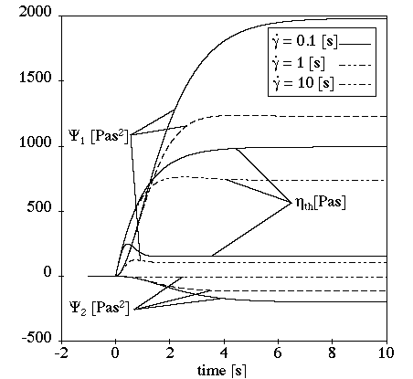
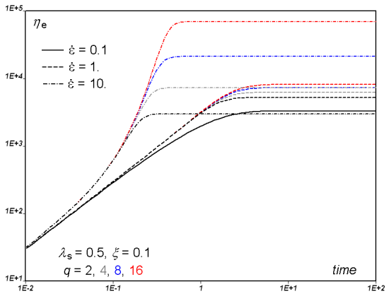
Finally, Figure 6.52: Effect of Parameter q on Transient Elongation Viscosity for Different
Values of the Elongation Rate shows the transient elongation viscosity of various
single-mode DCPP fluid model characterized by different branching levels
( ), at elongation rates
  successively equal to 0.1, 1 and 10. We find that all
curves collapse at low strain rate (0.1), while they markedly differ at high
strain rate (10).
successively equal to 0.1, 1 and 10. We find that all
curves collapse at low strain rate (0.1), while they markedly differ at high
strain rate (10).
Figure 6.52: Effect of Parameter q on Transient Elongation Viscosity for Different Values of the Elongation Rate
Elastomers are usually filled with carbon black and/or silicate. From the point of view of morphology, macromolecules at rest are trapped by particles of carbon black, via electrostatic van der Waals forces. Under a deformation field, electrostatic bonds can break, and macromolecules become free, while a reverse mechanism may develop when the deformation ceases. You can therefore be facing a macromolecular system consisting of trapped and free macromolecules, with a reversible transition from one state to the other one.
Leonov and Simhambhatla have developed a rheological model ([9], [10], [3]) for the simultaneous prediction of the behavior for trapped and free macromolecular chains. This model for filled elastomers involves actually two tensor quantities and a scalar one. These tensor quantities focus respectively on the behavior of the free and trapped macromolecular chains of the elastomer, while the scalar quantity quantifies the degree of structural damage (debonding factor). The model exhibits a yielding behavior. It is intrinsically nonlinear, as the nonlinear response develops and is observable at early deformations.
In a single-mode approach, the total stress tensor  can be decomposed as the sum of free and trapped
contributions, as follows:
can be decomposed as the sum of free and trapped
contributions, as follows:
 | (6–52) |
As for other viscoelastic models, a purely viscous component  is added to the viscoelastic components in order to get the
total extra-stress tensor:
is added to the viscoelastic components in order to get the
total extra-stress tensor:
 | (6–53) |
where  is the rate-of-deformation tensor and
  is the viscosity.
In Equation 6–52, subscripts
 and
and  respectively refer to the free and trapped parts. Each of
these contributions obeys its own equation. In particular, they invoke their own
deformation field described by means of Finger tensors.
respectively refer to the free and trapped parts. Each of
these contributions obeys its own equation. In particular, they invoke their own
deformation field described by means of Finger tensors.
An elastic Finger tensor  is defined for the free chains, which obeys the following
equation:
is defined for the free chains, which obeys the following
equation:
 | (6–54) |
where  is the relaxation time,
  is the unit tensor, while
  and
and  are the first invariant of
  and
and  , respectively, defined as
 | (6–55) |
 | (6–56) |
The implemented material function  that appears in Equation 6–54 is written as follows:
 | (6–57) |
The parameter  must be
  ; and increases slightly the amount of shear thinning.
Similarly, an elastic Finger tensor  is defined for the trapped chains, which obeys the following
equation:
is defined for the trapped chains, which obeys the following
equation:
 | (6–58) |
where  and
and  are the first invariant of
  and
and  , respectively, defined as
 | (6–59) |
 | (6–60) |
In the equation for the trapped chains, the variable  quantifies the degree of structural damage (debonding factor),
and is the fraction of the initially trapped chains that are debonded from the
filler particles during flow. The function
quantifies the degree of structural damage (debonding factor),
and is the fraction of the initially trapped chains that are debonded from the
filler particles during flow. The function  is a structural damage dependent scaling factor for the
relaxation time
is a structural damage dependent scaling factor for the
relaxation time  and is referred to as the “mobility function".
A phenomenological kinetic equation is suggested for  :
:
 | (6–61) |
In Equation 6–61,  is the local shear rate while
  is the yielding strain. Also,
  is a dimensionless time factor, which may delay or accelerate
debonding.
is a dimensionless time factor, which may delay or accelerate
debonding.
For the mobility function  appearing in Equation 6–58, the following form has been implemented:
 | (6–62) |
The above selection for the mobility function endows the rheological
properties with a yielding behavior. When  is large (or unbounded), the algebraic term dominates the
constitutive equation for
is large (or unbounded), the algebraic term dominates the
constitutive equation for  (Equation 6–58), and the solution is expected to be
  =1. When
  is vanishing,
  becomes governed by a purely transport equation; this may lead
to numerical troubles when solving a complex steady flow with secondary motions
(vortices). This situation can occur if parameter
becomes governed by a purely transport equation; this may lead
to numerical troubles when solving a complex steady flow with secondary motions
(vortices). This situation can occur if parameter  is set to zero and under no-debonding situation
(
is set to zero and under no-debonding situation
( ). Therefore, we suggest imposing a small (but nonzero) value
for parameter
). Therefore, we suggest imposing a small (but nonzero) value
for parameter  (by default, we suggest the value 0.05, which is a reasonable
compromise between rheological properties and solver stability). Based on this,
parameter
(by default, we suggest the value 0.05, which is a reasonable
compromise between rheological properties and solver stability). Based on this,
parameter  can be understood as the value of the mobility function under
no-debonding.
can be understood as the value of the mobility function under
no-debonding.
Finally, in order to relate the Finger tensors to the corresponding stress
tensor, potential functions are required. For  and
and  , the following expressions are suggested:
 | (6–63) |
 | (6–64) |
with  and
and  . It is interesting to note that
  has no effect on the shear viscosity, while it contributes to
a decrease of the elongational viscosity. On the other hand, the parameter
has no effect on the shear viscosity, while it contributes to
a decrease of the elongational viscosity. On the other hand, the parameter
 increases both shear and elongational viscosities. From there,
stress contributions from free and trapped chains in Equation 6–52 are respectively
given by:
increases both shear and elongational viscosities. From there,
stress contributions from free and trapped chains in Equation 6–52 are respectively
given by:
 | (6–65) |
 | (6–66) |
where parameter  is the initial ratio of free to trapped chains in the system.
A vanishing value of
is the initial ratio of free to trapped chains in the system.
A vanishing value of  indicates that all chains are trapped at rest, while a large
value of
indicates that all chains are trapped at rest, while a large
value of  indicates a system that essentially consists of free chains.
The units for the parameters and their names in the Ansys Polymat interface are as follows:
| Parameter | Name in Ansys Polymat | Mass | Length | Time |
|---|---|---|---|---|

| visc, additional viscosity | 1 | –1 | –1 |

| trelax, relaxation time | - | - | 1 |

| G, shear modulus | 1 | –1 | –2 |

| alpha, initial ratio of free to trapped chains | - | - | - |

|
beta, coefficient in
potential function

| - | - | - |

|
n, index in potential
function

| - | - | - |

| m, deformation history-dependence | - | - | - |

|
nu, power index
 in mobility function
| - | - | - |

| k, mobility under no-debonding | - | - | - |

| q, dimensionless time factor | - | - | - |

| gamma*, yielding strain | - | - | - |
 , ,  , ,  , , 
| - | 1 | –1 | –2 |

| - | - | - | –1 |

| - | - | - | - |
By default,  ,
,  ,
,  ,
,  , and
, and  are set to 1,
  and
and  are set to 2,
  is set to 0.05 and the other parameters to 0.
Important: In the current version of Ansys Polymat, you cannot fit the Leonov model and/or draw the corresponding rheometric curves in the chart.
From the point of view of rheology and numerical simulation, for single- and multi-mode fluid models, a purely viscous contribution must be added to the total extra-stress tensor. Actually, this is largely motivated by the fact that the matrix of the discretized system can be singular when all fields are initialized to values that correspond to the solution at rest. Hence, the first or only mode will always be accompanied by a Newtonian contribution, whose corresponding viscosity value received a unit default value. This value can be modified by the user.
Also, as suggested above, a non-vanishing value  should be selected for the mobility function under
no-debonding.
should be selected for the mobility function under
no-debonding.
As can be seen, next to parameters  and
and  controlling the linear properties, the model involves two
functions and several nonlinear parameters. In a single mode approach, the
influence of these parameters on the viscometric and elongational properties
can be easily identified, and appropriate values can be selected
accordingly. By default, the nonlinear parameters are assigned values that
are relevant from the point of view of rheology. In a multi-mode approach,
in order to facilitate the definition of a flow case, corresponding
nonlinear parameters should preferably be identical for each mode.
controlling the linear properties, the model involves two
functions and several nonlinear parameters. In a single mode approach, the
influence of these parameters on the viscometric and elongational properties
can be easily identified, and appropriate values can be selected
accordingly. By default, the nonlinear parameters are assigned values that
are relevant from the point of view of rheology. In a multi-mode approach,
in order to facilitate the definition of a flow case, corresponding
nonlinear parameters should preferably be identical for each mode.
In simple shear flow, the Leonov model exhibits shear thinning, which is
slightly affected by some parameters. Figure 6.53: Shear Viscosity of the Leonov Model with Parameters G=1000, λ=1,
q=1, β=0, ν=2, γ*=2, and a=1, k=n=m=0 (continuous
lines). shows
that an increase of the parameter  (initial ratio of free to trapped chains) slightly
decreases the shear viscosity at low shear rates. This can be easily
understood if you consider, for example, that when
(initial ratio of free to trapped chains) slightly
decreases the shear viscosity at low shear rates. This can be easily
understood if you consider, for example, that when  =0, the material consists only of trapped chains at rest.
The figure also shows that parameter
=0, the material consists only of trapped chains at rest.
The figure also shows that parameter  increases the shear viscosity at high shear rates, while
parameter
increases the shear viscosity at high shear rates, while
parameter  has a very limited influence. Finally, as can be seen in
Figure 6.53: Shear Viscosity of the Leonov Model with Parameters G=1000, λ=1,
q=1, β=0, ν=2, γ*=2, and a=1, k=n=m=0 (continuous
lines).,
shear viscosity curves do not show a plateau at low shear rates. This is the
fingerprint of the yielding behavior of the fluid model, which is controlled
by the value of the mobility function under no-debonding (parameter
has a very limited influence. Finally, as can be seen in
Figure 6.53: Shear Viscosity of the Leonov Model with Parameters G=1000, λ=1,
q=1, β=0, ν=2, γ*=2, and a=1, k=n=m=0 (continuous
lines).,
shear viscosity curves do not show a plateau at low shear rates. This is the
fingerprint of the yielding behavior of the fluid model, which is controlled
by the value of the mobility function under no-debonding (parameter
 ). Actually, if
  increases, the viscosity curves exhibit a plateau at low
shear rates; however, as can be seen in the insert, this does not affect the
behavior at high shear rates, while it may improve the stability of the
solver.
increases, the viscosity curves exhibit a plateau at low
shear rates; however, as can be seen in the insert, this does not affect the
behavior at high shear rates, while it may improve the stability of the
solver.
Figure 6.53: Shear Viscosity of the Leonov Model with Parameters G=1000, λ=1, q=1, β=0, ν=2, γ*=2, and a=1, k=n=m=0 (continuous lines).
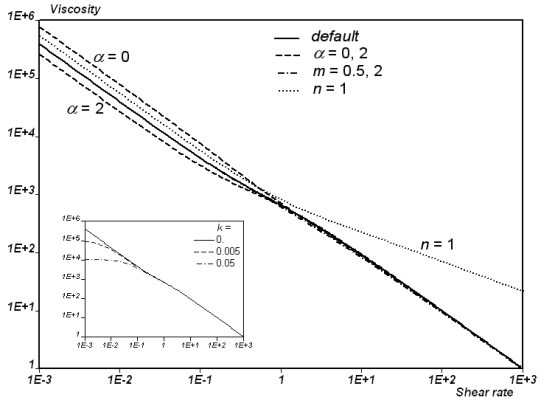
Dashed and dashed-dotted lines show the viscosity for the value of the parameters as indicated. The insert shows the viscosity curves obtained for various values of the mobility function under no-debonding (parameter k). Note that these curves are not obtained from Ansys Polymat; they result from semi-analytical calculations.
Figure 6.54: First Normal Stress Difference of the Leonov Model with Parameters
G=1000, λ=1, q=1, β=0, ν=2, γ*=2, and a=1, k=n=m=0
(continuous lines). shows
that similar trends are found for the first normal stress difference. Figure 6.54: First Normal Stress Difference of the Leonov Model with Parameters
G=1000, λ=1, q=1, β=0, ν=2, γ*=2, and a=1, k=n=m=0
(continuous lines). shows
that an increase of the parameter  slightly decreases the first normal stress difference at
all shear rates. The figure also shows that parameter
slightly decreases the first normal stress difference at
all shear rates. The figure also shows that parameter  increases the first normal stress difference at all shear
rates, while parameter
increases the first normal stress difference at all shear
rates, while parameter  decreases it at high shear rates. Finally, as can be seen,
the first normal stress difference shows a plateau at low shear rates; this
is a counterpart of the yielding behavior of the fluid model, which is also
controlled by the value of the mobility function under no-debonding
(parameter
decreases it at high shear rates. Finally, as can be seen,
the first normal stress difference shows a plateau at low shear rates; this
is a counterpart of the yielding behavior of the fluid model, which is also
controlled by the value of the mobility function under no-debonding
(parameter  ). Actually, if
  increases, the first normal stress difference exhibit a
quadratic behavior at low shear rates; however, as can be seen in the
insert, this does not affect the behavior at high shear rates, while it may
improve the stability of the solver.
increases, the first normal stress difference exhibit a
quadratic behavior at low shear rates; however, as can be seen in the
insert, this does not affect the behavior at high shear rates, while it may
improve the stability of the solver.
Figure 6.54: First Normal Stress Difference of the Leonov Model with Parameters G=1000, λ=1, q=1, β=0, ν=2, γ*=2, and a=1, k=n=m=0 (continuous lines).
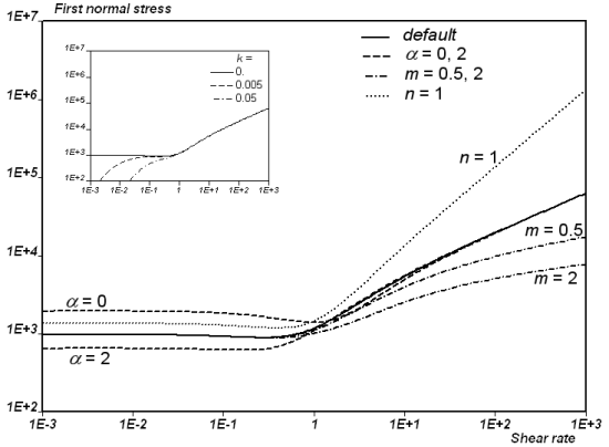
Dashed, dashed-dotted and dotted lines show the first normal stress
difference for the value of the parameters as indicated. The insert shows
the curves of first normal stress difference obtained for various values of
the mobility function under no-debonding (parameter  ). Note that these curves are not obtained from Ansys Polymat;
they result from semi-analytical calculations.
). Note that these curves are not obtained from Ansys Polymat;
they result from semi-analytical calculations.
In simple elongation flow, the Leonov model exhibits marked strain
thinning at low strain rates; it is slightly affected by some parameters.
Figure 6.55: Elongation Viscosity of the Leonov Model with Parameters G=1000,
λ=1, q=1, n=1, ν=2, γ*=2, and a=1, β=k=m=0 (continuous
lines). shows that an increase of the parameter  (initial ratio of free to trapped chains) slightly
decreases the elongation viscosity at low strain rates. This can be easily
understood if you consider, for example, that when
(initial ratio of free to trapped chains) slightly
decreases the elongation viscosity at low strain rates. This can be easily
understood if you consider, for example, that when  =0, the material consists only of trapped chains at rest.
The figure also shows that parameter
=0, the material consists only of trapped chains at rest.
The figure also shows that parameter  increases the elongation viscosity at high strain rates,
while parameters
increases the elongation viscosity at high strain rates,
while parameters  and
and  decrease the elongation viscosity. Finally, as can be seen
in Figure 6.55: Elongation Viscosity of the Leonov Model with Parameters G=1000,
λ=1, q=1, n=1, ν=2, γ*=2, and a=1, β=k=m=0 (continuous
lines)., elongation viscosity curves do not show a plateau. This is the
fingerprint of the yielding behavior of the fluid model, which is controlled
by the value of the mobility function under no-debonding (parameter
decrease the elongation viscosity. Finally, as can be seen
in Figure 6.55: Elongation Viscosity of the Leonov Model with Parameters G=1000,
λ=1, q=1, n=1, ν=2, γ*=2, and a=1, β=k=m=0 (continuous
lines)., elongation viscosity curves do not show a plateau. This is the
fingerprint of the yielding behavior of the fluid model, which is controlled
by the value of the mobility function under no-debonding (parameter
 ). Actually, if
  increases, the elongation viscosity curves exhibit a
plateau at low strain rates; however, as can be seen in the insert of Figure 6.55: Elongation Viscosity of the Leonov Model with Parameters G=1000,
λ=1, q=1, n=1, ν=2, γ*=2, and a=1, β=k=m=0 (continuous
lines).,
this does not really affect the behavior at high strain rates while it may
improve the stability of the solver.
increases, the elongation viscosity curves exhibit a
plateau at low strain rates; however, as can be seen in the insert of Figure 6.55: Elongation Viscosity of the Leonov Model with Parameters G=1000,
λ=1, q=1, n=1, ν=2, γ*=2, and a=1, β=k=m=0 (continuous
lines).,
this does not really affect the behavior at high strain rates while it may
improve the stability of the solver.
Figure 6.55: Elongation Viscosity of the Leonov Model with Parameters G=1000, λ=1, q=1, n=1, ν=2, γ*=2, and a=1, β=k=m=0 (continuous lines).
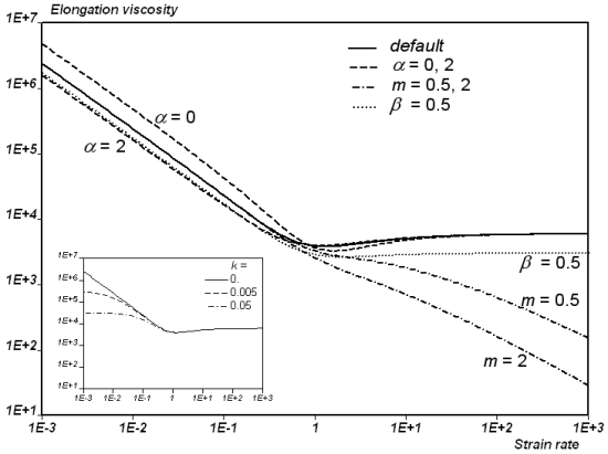
Dashed, dashed-dotted and dotted lines show the elongation viscosity for
the value of the parameters as indicated. The insert shows the curves of the
steady elongation viscosity obtained for various values of the mobility
function under no-debonding (parameter  ). Note that these curves are not obtained from Ansys Polymat;
they result from semi-analytical calculations.
). Note that these curves are not obtained from Ansys Polymat;
they result from semi-analytical calculations.
Figure 6.56: Transient Shear Viscosity of the Leonov Model Versus Time, at Shear
Rates Ranging from 10^-2 to 10, With Parameters G=1000, λ=1, q=1,
n=1, β=0, ν=2, γ*=2, and a=1, k=m=n=0, (continuous
lines).
shows the transient shear viscosity versus time at shear rates ranging from
10-2 to 10, for various values of parameters
 and
and  . At first, as can be seen, the transient shear viscosity
exhibits an overshoot before reaching the steady value. It is also
interesting to note that the response time decreases when the shear rate
increases. This actually results from the increasing mobility function under
increasing shear rates. Eventually, we find that parameter
. At first, as can be seen, the transient shear viscosity
exhibits an overshoot before reaching the steady value. It is also
interesting to note that the response time decreases when the shear rate
increases. This actually results from the increasing mobility function under
increasing shear rates. Eventually, we find that parameter  decreases the elongation viscosity, while the other
parameters have a somewhat less marked influence.
decreases the elongation viscosity, while the other
parameters have a somewhat less marked influence.
Figure 6.56: Transient Shear Viscosity of the Leonov Model Versus Time, at Shear Rates Ranging from 10^-2 to 10, With Parameters G=1000, λ=1, q=1, n=1, β=0, ν=2, γ*=2, and a=1, k=m=n=0, (continuous lines).
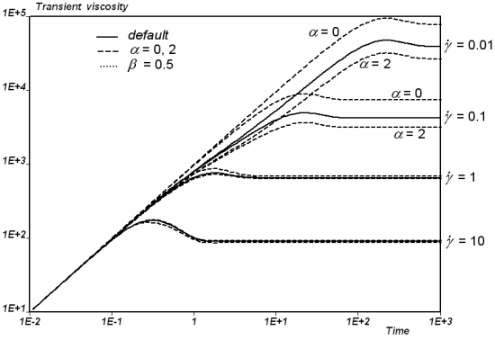
Dashed and dotted lines show the viscosity for the value of the parameters as indicated. Note that these curves are not obtained from Ansys Polymat; they result from semi-analytical calculations.