


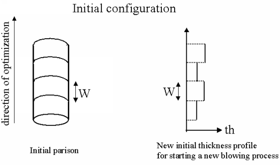
This new postprocessor is available for blow molding and thermoforming processes in shell models. Due to some constraints on thickness distribution of the final product, the thickness distribution of the initial parison or of the initial sheet of polymer is estimated, which will eventually provide the required thickness distribution. The procedure is iterative. Start with your specified initial thickness distribution and run the simulation. At the end of it, the postprocessor is activated and a file is generated containing a new initial distribution. Then, run a new simulation with this new initial thickness distribution. Repeat this procedure for 5 to 10 optimization steps until the solution is converged. The final thickness obtained will be very close to the requested profile and with a minimum of mass.
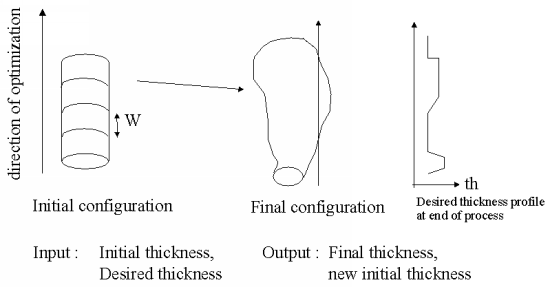
Define your blow molding simulation with a specified initial thickness distribution. Then create the "parison programming" postprocessor.
Create a new sub-task.
 Create a sub-task
Select Postprocessor as the sub-task type.
Postprocessor
When prompted, enter a name for the postprocessor sub-task.
In the F.E.M. Task Postprocessor menu, select Parison programming.
Parison programming
Select the layer on which the thickness distribution will be optimized. Select thickness optimisation DISABLED for layer my_layer. By default, the optimization for the layer my_layer will be disabled. To activate the menu for optimization, select:
Enable optimisation
Specify the direction of optimization. Select Modify the direction Z of optimisation.
The direction mentioned here is the direction of extrusion of parison in a blow molding simulation. In a thermoforming simulation, it is the direction transverse to the extrusion direction of the polymer sheet.
Specify the under-relaxation factor
 . Select Modify the under-relaxation
factor.
. Select Modify the under-relaxation
factor. As the technique of optimization is iterative, it is mandatory to specify an under-relaxation factor (
 ) to avoid oscillations in the solution for each step.
 ranges between 0 and 1 and has a default value of
0.9.Specify the width of the stripes. Select Modify the width of stripes.
You have two alternatives:
If the width of the stripes is set to zero, then for each nodal value, a new thickness is evaluated, in order to obtain for that node, at the end of blowing simulation, a specific desired thickness.

(17–31)
where
 is the index of the current node of the
parison/sheet,
is the index of the current node of the
parison/sheet,  is the initial thickness at that node,
 is the requested thickness for that node, and
 is its final thickness.
 If the width of the stripes is set to W (W>0), then you will evaluate one constant initial thickness for each stripe of the parison/sheet, that is, for each node, you will estimate its new initial thickness (see Equation 17–31) and determine in which stripe it is included. The new initial thickness of the stripe
 will then be:
(17–32)
Specify the time of activation of the postprocessor. Select Modify the time of activation.
The new initial thickness distribution is calculated at the end of the simulation, not in the beginning. It is recommended that you specify the time of activation as
 the time of simulation.
 Specify the required thickness distribution (piecewise linear) in the direction of optimization.
Modify the list of pairs (Z, h)
The new initial thickness distribution is saved in a CSV file. This makes it easier for the next step of optimization, where you have to reread the data file and change the initial thickness in the blow molding sub-task.
Modify the CSV filename = new_initial_thickness.csv
The result of the postprocessor is shown in Figure 17.10: Final Result.
Several new fields appear in the Field management menu at the end of the Ansys Polydata session:
THICKNESS: This field is evaluated by the shell model. It changes as the blowing process advances.
THICKNESS INI: This is the initial thickness used to start the simulation.
THICKNESS DES: This is the desired thickness profile at the end of the blowing process.
THICKNESS NEW: This is the new initial thickness distribution evaluated by the postprocessor. This field is saved in a CSV file that will be used at the next step of optimization, to initialize the thickness field at time t=0.
Note: The last three fields carry a value equal to zero until the simulation reaches the time of activation. For the remaining time of the simulation, the postprocessor determines the values of the fields. Only the last CSV file should be used to start a new optimization step.