You can apply deformation methods on lines to define the boundary conditions of a surface in a domain on which the elastic remeshing method has been applied. You have the following options for deforming or moving lines:
free line
The "free line" method does not apply an equation on the line. The coordinates of the nodes belonging to this line are governed by the equations applied on the 2D domain that contains this line.
elastic remeshing
For the "elastic remeshing" method, the motion of the nodes is governed by Equation 35–3. The pseudo-elastic equation defined on this line replaces the 2D equation for the interior nodes of the line. This equation also requires boundary conditions, which can be selected from the point displacement methods described in Point Displacement.
line deformation
For the "line deformation" method, the motion of each node is governed by the equation used for the rigid translation method (Equation 35–2). But the line deformation method differs from the rigid translation method, in that the displacement direction and amplitude need not be uniform for all the nodes. The amplitude
 and the component direction
  are given by second order differential equations:
(35–10)
and

(35–11)
where
 is the Laplace operator.
 From a mathematical point of view, Equation 35–10 and Equation 35–11
 and one value for
  in order to yield a solution (you may define more). At
these points
in order to yield a solution (you may define more). At
these points 
(35–12)
and

(35–13)
where
 and
and  are the values you defined for the amplitude and the
direction components, respectively.
are the values you defined for the amplitude and the
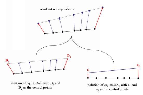
direction components, respectively. The nodes where you defined the direction and/or the displacement amplitude are referred to as the "control points". The result of Equation 35–10 and Equation 35–11 is a linear variation between two successively defined values. Figure 35.6: The Motion of Nodes due to the Line Deformation Method shows the solution of Equation 35–11 for the direction with
 and
and  for the boundary conditions (left bottom), the solution of
Equation 35–10 for the
displacement amplitude with
for the boundary conditions (left bottom), the solution of
Equation 35–10 for the
displacement amplitude with  and
and  for the boundary conditions (bottom right), and the
solution of Equation 35–2 with
the new node positions (top).
for the boundary conditions (bottom right), and the
solution of Equation 35–2 with
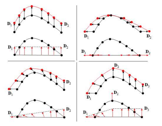
the new node positions (top). This method can also be applied on curved lines. For curved lines, note that Equation 35–11 does not take the curvature into account, and the direction vectors are not the normal vectors to the curve.
Figure 35.7: The Line Deformation Method on a Curved Line shows examples of different direction vectors
 ,
,  , and
, and  imposed on a curved line, with the displacement amplitude
set to 1. For each case, the lower portion of the figure depicts the initial
curve and the directions computed on the basis of
imposed on a curved line, with the displacement amplitude
set to 1. For each case, the lower portion of the figure depicts the initial
curve and the directions computed on the basis of  ,
,  , and
, and  , while the upper portion shows the resultant node
positions.
, while the upper portion shows the resultant node
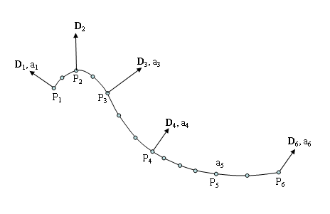
positions. You do not have to impose a value on both the direction and amplitude for a given node. In other words, you can impose a value for one, or the other, or both, as shown in Figure 35.8: The Line Deformation Method with Multiple Control Points.
The following is a description of the amplitude and direction components on the nodes between
 and
and  in Figure 35.8: The Line Deformation Method with Multiple Control Points. The direction components vary linearly between node
  and node
  (ranging from
  to
to  ), as well as between node
  and node
  (ranging from
  to
to  ). The amplitude values, on the other hand, vary linearly
between node
). The amplitude values, on the other hand, vary linearly
between node  and node
  (ranging from
  to
to  ), as there is no imposed amplitude at node
  . A similar description could be made for the nodes between
 and
and  , which have imposed amplitude values at
  ,
,  , and
, and  , but have direction components only imposed at
 and
and  .
. It is recommended that the line deformation method not be used on lines that are made of several disconnected parts. Such a circumstance can arise, for example, when a line is defined by the intersection of two surfaces that meet in separate locations. If you do decide to use the line deformation method for such a line, then you must define at least one control point on each of the disconnected parts.
In order to provide you with flexibility when defining the point displacement, the direction you specify does not need to be normalized. Still, it is recommended that you specify unit vectors for the control points, as this can lead to better control.
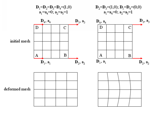
If you want a control point in a line to be fixed, it is recommended that you set the amplitude value equal to 0. You could also accomplish this by setting the direction equal to the null vector. Figure 35.9: Mesh Deformation Including Fixed Points illustrates the results of both methods on a line that belongs to a surface, on which is applied the elastic remeshing method.
On the left side of the Figure 35.9: Mesh Deformation Including Fixed Points, a unit vector (1,0) is imposed for the four directions
 ,
,  ,
,  , and
, and  at control points A, B, C, and D, respectively. The
amplitude is set to 0 at points A and D, and set to 1 at points B and C. The
resultant displacement is then 0 along line AD, and the vector (1,0) along
line BC. For the nodes in lines AB and DC, the direction is constant (1,0)
and the amplitude displacement varies linearly from 0 (points A and D) to 1
(points B and C). Hence, the resulting displacement varies linearly along
lines AB and DC.
at control points A, B, C, and D, respectively. The
amplitude is set to 0 at points A and D, and set to 1 at points B and C. The
resultant displacement is then 0 along line AD, and the vector (1,0) along
line BC. For the nodes in lines AB and DC, the direction is constant (1,0)
and the amplitude displacement varies linearly from 0 (points A and D) to 1
(points B and C). Hence, the resulting displacement varies linearly along
lines AB and DC. The settings for the control points on the right side of Figure 35.9: Mesh Deformation Including Fixed Points are similar, except that the null vector (0,0) is imposed for the directions
 and
and  at points A and D, respectively. While the resultant
displacements along lines AD and BC are the same as on the left side of the
figure, they are different along lines AB and DC. For lines AB and DC, the
x-component of the direction varies linearly from 0 to 1, while at the same
time the amplitude displacement varies linearly from 0 to 1. The resultant
displacement is therefore no longer linear along AB and DC, and the nodes
are not equidistant. Note that the interior nodes behave differently than
the nodes of line AB and DC, as the elastic remeshing method attempts to
respect the initial distribution.
at points A and D, respectively. While the resultant
displacements along lines AD and BC are the same as on the left side of the
figure, they are different along lines AB and DC. For lines AB and DC, the
x-component of the direction varies linearly from 0 to 1, while at the same
time the amplitude displacement varies linearly from 0 to 1. The resultant
displacement is therefore no longer linear along AB and DC, and the nodes
are not equidistant. Note that the interior nodes behave differently than
the nodes of line AB and DC, as the elastic remeshing method attempts to
respect the initial distribution. rigid translation
For the "rigid translation" method, the motion of the nodes is governed by Equation 35–2. This method is applied on all topological entities included in the domain definition (that is, points). Hence, it is not possible to apply another motion on these points when defining the deformation of an adjacent domain.
fixed surface
For the "fixed surface" method, the motion of the nodes is governed by Equation 35–1. As a result, all the nodes of the surface remain fixed at their original coordinates. This method is applied on all topological entities included in the domain definition (that is, points). Hence, it is not possible to apply another motion on these points when defining the deformation of an adjacent domain.
symmetry
For the "symmetry" method, a straight line on a 2D geometry is treated as a line of symmetry. In other words, the line is deformed due to the methods applied on its extremities, with the constraint that the nodes remain in the original line. Note that the selection of the symmetry method for line deformation does not define the flow as symmetrical about this line, as the two conditions are not linked.