For 2D and 3D viscoelastic flow, the standard differential viscoelastic models can be used for both isothermal and non-isothermal flows. For shell models, the simplest rheological description consists of selecting a constant viscosity. In some situations it is more desirable to define a simple viscosity model whose magnitude depends on the local strain.
The fluid constitutive equation is written as follows:
 | (17–7) |
Here the viscosity  depends on the local strain or deformation
  , which is locally evaluated on the basis of the stretching
undergone by the individual elements with respect to their initial configuration.
The relevance of this model lies in the fact that it enables a differentiated
behavior as a function of the accumulated deformation. The advantage is that the
property can be easily measured in a simple traction experiment or with a simple
elongation rheometer.
, which is locally evaluated on the basis of the stretching
undergone by the individual elements with respect to their initial configuration.
The relevance of this model lies in the fact that it enables a differentiated
behavior as a function of the accumulated deformation. The advantage is that the
property can be easily measured in a simple traction experiment or with a simple
elongation rheometer.
In a simple traction experiment, a (usually dog-bone shaped) sample of initial
length  is stretched at a constant stretching velocity
  and the tensile stress is recorded as a function of the
deformation. Data manipulation allows converting this data into a viscosity versus
deformation, by taking the viscosity
and the tensile stress is recorded as a function of the
deformation. Data manipulation allows converting this data into a viscosity versus
deformation, by taking the viscosity  as the ratio of the stress to the strain rate
  given by
 | (17–8) |
where  is the actual deformation. It is therefore possible to extract the
curve
is the actual deformation. It is therefore possible to extract the
curve  . A simple traction experiment is appealing for thermoforming
applications, as the sample can be stretched at a rather low temperature. Despite
the simplicity, the model embraces possible morphological changes, such as strain
induced crystallization.
. A simple traction experiment is appealing for thermoforming
applications, as the sample can be stretched at a rather low temperature. Despite
the simplicity, the model embraces possible morphological changes, such as strain
induced crystallization.
For extrusion blow molding applications, where the parison is inflated right after
extrusion, it is probably more appropriate to consider a viscosity measurement using
a simple elongation rheometer. Here, the sample is usually stretched at a constant
strain rate  , and the viscosity is given as a function of time. Here again,
data manipulation allows converting this measurement into a viscosity versus
deformation, by converting the time into a deformation. Typically, the Cauchy
deformation
, and the viscosity is given as a function of time. Here again,
data manipulation allows converting this measurement into a viscosity versus
deformation, by converting the time into a deformation. Typically, the Cauchy
deformation  is given by
 | (17–9) |
Since blow molding occurs under relatively fast deformations, it is appropriate to consider the curve data obtained under high strain rate.
Fitting the viscosity-deformation curve is mainly a matter of algebra and three functions are available to facilitate this task.
The first function is a deformation independent viscosity
 , which requires just one parameter.
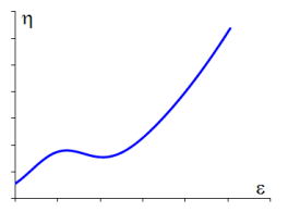
The second function is the sum of a parabola plus a Gaussian function, which can be written as:

(17–10)
This function combines a monotonic increase with a hump centered around
 and whose width is given by
  . This function can be interesting when on-going
crystallization is subsequent to strain-thinning. Take care to ensure that
all properties have positive values. In particular,
. This function can be interesting when on-going
crystallization is subsequent to strain-thinning. Take care to ensure that
all properties have positive values. In particular,  ,
,  and
and  must be positive. Figure 17.2: Typical Viscosity Curve Exhibiting Strain Hardening shows a typical
viscosity described by this law.
must be positive. Figure 17.2: Typical Viscosity Curve Exhibiting Strain Hardening shows a typical
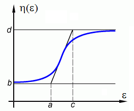
viscosity described by this law.A third function is a smoothed ramp, described by means of four parameters. Qualitatively, the property increases from values
 to
to  when the deformation varies from
  to
to  . Here you must also ensure that all properties have
positive values. In particular,
. Here you must also ensure that all properties have
positive values. In particular,  and
and  must be positive. Figure 17.3: Typical Viscosity Curve Described with the Smooth Ramp shows a typical
viscosity described by this law.
must be positive. Figure 17.3: Typical Viscosity Curve Described with the Smooth Ramp shows a typical
viscosity described by this law.