


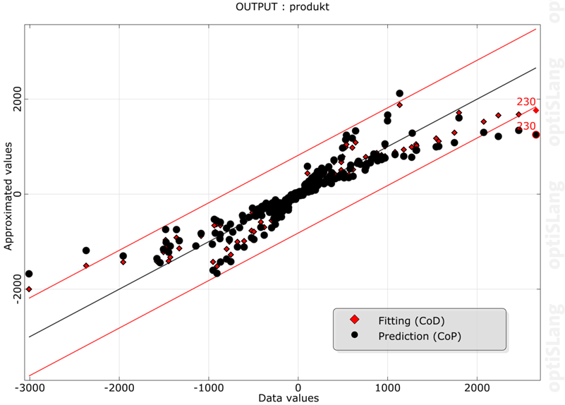
If the data set contains cross-validation values generated by the MOP, they can be displayed using this plot. Prediction (cross-validation) and fitting (CoD) values are displayed together, to illustrate the quality of prediction. This plot can be useful to identify and deactivate outliers and, as a result, improve the quality of prognosis of the surrogate models.
The residual plot has four different modes which can be selected in the plot settings:
Values: Shows the predicted and fitting values versus the original data values
Errors: Shows the predicted error and fitting error values versus the original values
Absolute Errors: Shows the absolute predicted error and absolute fitting error values versus the original values
Sample CoPs: Shows the contribution of each sample to the global CoP, the mean of all sample CoPs is the global CoP value
If the values are shown, the diagonal represents the perfect model which means that the predicted or fitted values are equal to the original data values. This corresponds to the horizontal line at zero when showing the error values. The error ranges (red lines) are scaled by the standard deviation (root mean square error) of the prediction error values (predicted minus original values) times the user-defined sigma level.
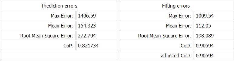
Statistical Data
This section of the plot displays additional information about statistic values (maximum, mean, rms) of the two different sets of error values, and can be compared. The CoP and the CoD of the currently selected model is also shown here.
Settings
| Option | Description |
|---|---|
| Common Settings | |
| Show ordinate as | Select one of the following:
|
| Sigma level | The plot displays the mean line plus two sigma lines. This value defines the distance between them. |
| Preferences | |
|
The following preference settings are available:
For more details, see Plot Preference Settings. | |
Python scripting
Create Visual
Creates an Residual plot using data with data_id
residual_plot = Visuals.Residual(Id("Residual plot"), data_id )
Add to Postprocessing
Adds Residual plot in postprocessing to control_container, using the specified relative positioning.
    control_container.add_control (
        residual_plot,
        True,
        RELATIVE_POSITIONING,
        1/2., 0, 1/2., 1/2.
    )