


This tutorial allows you to complete a robustness evaluation of a single degree-of-freedom system excited with initial kinetic energy.
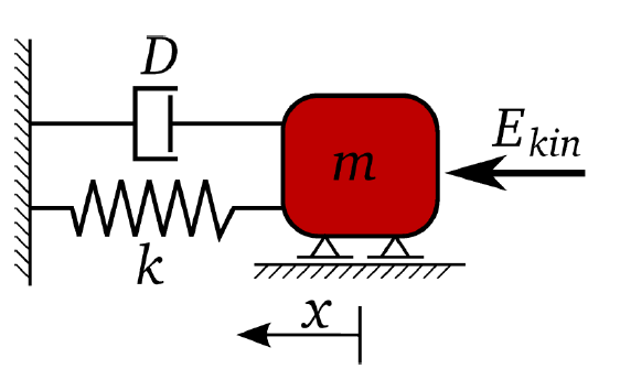
You will complete a robustness evaluation at the deterministic optimum.

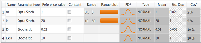
Mass m, damping ratio D, stiffness k and initial kinetic energy Ekin are taken as normally distributed random variables.

In this tutorial, you complete the robustness evaluation using the optiSLang extension in Workbench.
This tutorial demonstrates how to do the following:
Define the random input variables
Complete a robustness analysis with respect to damped eigen frequency and maximum amplitude
Check the coefficient of variation of the objective and constraints
Check if the safety constraint
 is outside of the 4.5σ level
Check the importance of input variables
Check explainability by using the Metamodel of Optimal Prognosis (MOP) and Coefficients of Prognosis (CoP)
Iterate the constraints manually until the criteria are fulfilled
You must complete the Optimization of a Damped Oscillator in Ansys Workbench tutorial before starting this one.
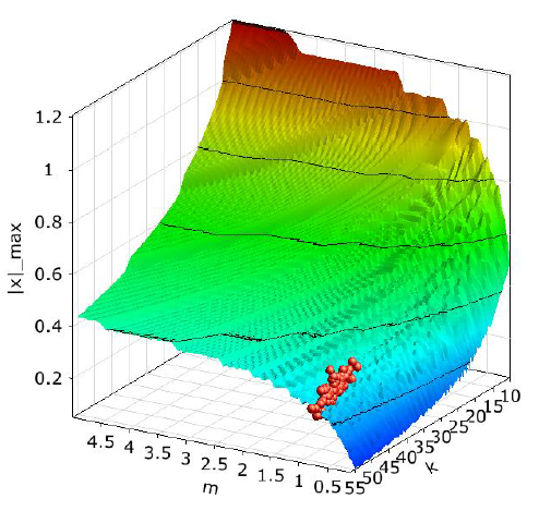
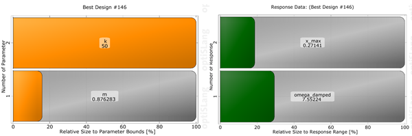
The best design of the Adaptive Metamodel of Optimal Prognosis (AMOP) optimization is used as the reference for the robustness analysis.
To set up and run the tutorial, perform the following steps:
Start Workbench.
From the menu bar, select > .
Browse to the location of the damped oscillator optimization Workbench project used in the previous tutorial
Click .
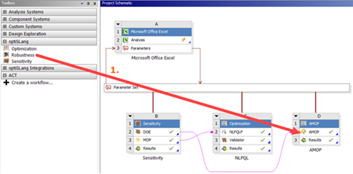
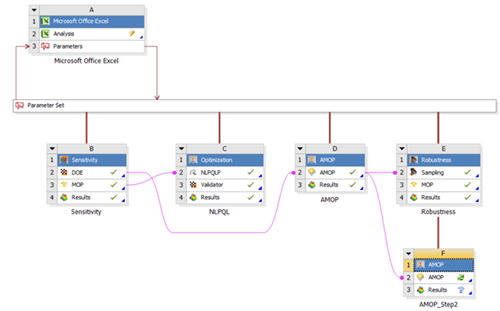
Drag the Robustness wizard from the Toolbar and drop it onto the AMOP cell of the AMOP system.
In rows 3 and 4 (D and Ekin), clear the Constant check box.
In row 1 (m), double-click the Parameter type cell and select from the drop-down list.
Repeat step 3 for row 2 (k).
In row 3 (D) double-click the Parameter type cell and select from the drop-down list.
Repeat step 5 for row 4 (Ekin).
Double-click the CoV cell for each row and change the values to the following:
Row 1 (m):
2%Row 2 (k):
5%Row 3 (D):
10%Row 4 (Ekin):
10%
Click .
Do not adjust or add to the currently displayed values for parameters, responses, and criteria.
Click .
Do not adjust the current robustness/reliability method settings.
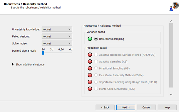
Click .
Do not adjust the current algorithm settings.
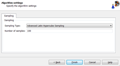
Click .
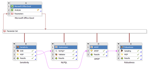
The Robustness system is added to the Project Schematic.
To save the current project, from the menu bar, select > or from the main toolbar, click
 .
.Right-click the Results cell of the Robustness system and select from the context menu.
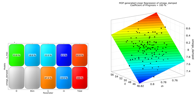
The results of the robustness evaluation are displayed. You can observe:
Both responses show almost linear behavior
omega_damped can be explained very well by m and k
x_max is mainly influenced by D, k and Ekin and has a lower CoP as in the design space due to locally more dominant solver noise
In the Monitoring pane, select > > .
Select >
Double-click the Upper cell under Failure Limit for omega_damped and enter
8.5.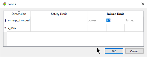
Click .
Under Common settings, select as the first variable.
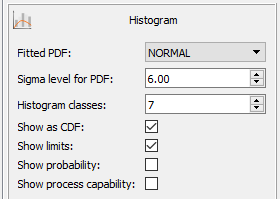
In the Show settings for list, select .
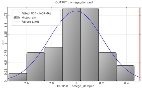
In the Fitted PDF list, select .
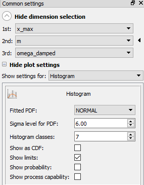
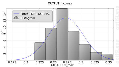
Review the resulting graph.
Histogram and fitted PDF agree well.
Under the histogram, expand .
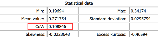
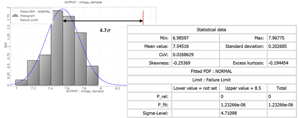
Review the statistical data. You can observe:
Mean is not close to deterministic value
CoV is larger as maximum input variation (10%)
Optimum is not robust in terms of the objective function
Under Common settings, select as the first variable.
In the Show settings for list, select .
In the Fitted PDF list, select .
Review the resulting graph.
Histogram and fitted PDF agree well.
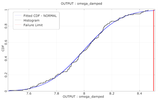
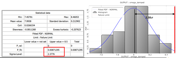
In the histogram settings, select the Show as CDF check box.
Review the resulting graph.
Empirical and fitted normal CDF agree well. Estimation of the failure probability by assuming a normal distribution seems reasonable.
Under the fitted CDF graph, expand .
Review the statistical data. You can observe:
Safety margin is only 2.38σ, which corresponds to a 1% failure probability
Optimum is not robust in terms of the constraint condition
To perform iterative robust design optimization:
Modify the design by reducing the mean of omega_damped by an additional deterministic optimization
Consider all previous optimization designs for the new optimization
Check the robustness again
The deterministic constraint for the second optimization step, assuming a constant standard deviation:
Mean value + 4.5 * standard deviation ≤ 8.5 rad/s
Mean omega_damped ≤ 7.6
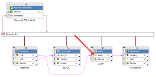
Drag the Optimization wizard from the Toolbar and drop it onto the AMOP cell of the AMOP system.
In the Limit field for the omega_damped constraint, enter
7.6.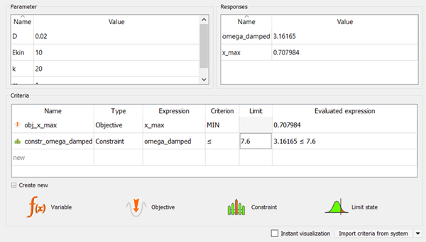
Change the solver type to .
Leave the optimization method as Adaptive Metamodel of Optimal Prognosis (AMOP).
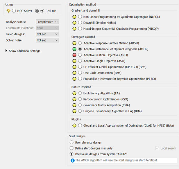
Click .
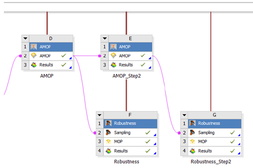
A second AMOP system is added to the Project Schematic.
Double-click the second AMOP system name or right-click the system header and select from the context menu.
Type
AMOP_Step2.Press Enter.
Double-click the AMOP cell of the AMOP_Step2 system to open the settings.
On the Adaption tab, select the Show advanced settings check box.
In the Maximum number of samples field, enter
45.Adjust the refinement sliders so the first two are at 0% and the Importance of optimization criteria slider is at 100%
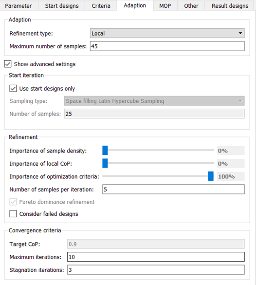
To save and close the settings, click .
To save the current project, from the menu bar, select > or from the main toolbar, click
.Right-click the Results cell of the AMOP_Step2 system and select from the context menu.
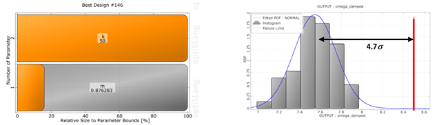
The optimizer increases the mass. The best design of the second AMOP optimization is considered automatically as nominal design of the robustness analysis.
Drag the Robustness wizard from the Toolbar and drop it onto the AMOP cell of the AMOP_Step2 system.
At the bottom of the Parametrize Inputs table, click
From the Select system pane, select Robustness.
To highlight all of the parameters in the table, do one of the following:
Click the name of the first parameter, press Shift, and then click the name of the parameter the last row.
Click the name of the first parameter, then with the mouse key pressed, pull down to the last parameter and release the mouse key.
Click .
The selected parameters are imported.
Click .
Do not adjust or add to the currently displayed values for parameters, responses, and criteria.
Click .
Do not adjust the current robustness/reliability method settings.
Click .
Do not adjust the current algorithm settings.
Click .
A second Robustness system is added to the Project Schematic.
Double-click the second Robustness system name or right-click the system header and select from the context menu.
Type
Robustness_Step2.Press Enter.
To save the current project, from the menu bar, select > or from the main toolbar, click
.Right-click the Results cell of the Robustness_Step2 system and select from the context menu.
The safety margin of omega_damped is now 4.7σ, which corresponds to a failure probability of about 1.2x10⁻⁶, if the response is perfectly normally distributed.
This manual iteration has found a robust optimum within two iterations.
| Optimization (Global ARSM) | Robustness (100 ALHS) | ||||||
|---|---|---|---|---|---|---|---|
| Constraint | m | k | ω | Xmax | Mean ω | Sigma ω | Sigma Level |
| ω ≤ 8 | 0.79 | 50 | 7.96 | 0.26 | 7.99 | 0.21 | 2.4 |
| ω ≤ 7.6 | 0.87 | 50.0 | 7.56 | 0.27 | 7.55 | 0.20 | 4.7 |